
[1]:
# This information helps with debugging and getting support :)
import sys, platform
import pandas as pd
import bifacial_radiance as br
print("Working on a ", platform.system(), platform.release())
print("Python version ", sys.version)
print("Pandas version ", pd.__version__)
print("bifacial_radiance version ", br.__version__)
Working on a  Windows 10
Python version  3.11.8 | packaged by conda-forge | (main, Feb 16 2024, 20:40:50) [MSC v.1937 64 bit (AMD64)]
Pandas version  2.2.3
bifacial_radiance version  0.5.0b2.dev4+gedb973d.d20250924
8 - Electrical Mismatch Method (sorry, this tutorial is deprecated and non-functional as of v0.5.0)#
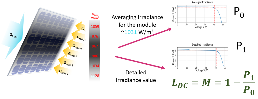
Nonuniform rear-irradiance on bifacial PV systems can cause additional mismatch loss, which may not be appropriately captured in PV energy production estimates and software.
The analysis.py module in bifacial_radiance comes with functions to calculate power output, electrical mismatch, and some other irradiance calculations. This is the procedure used for this proceedings and submitted journals, which have much more detail on the procedure.
Deline, C., Ayala Pelaez, S., MacAlpine, S., Olalla, C. Estimating and Parameterizing Mismatch Power Loss in Bifacial Photovoltaic Systems. Progress in PV 2020, https://doi.org/10.1002/pip.3259
Deline C, Ayala Pelaez S, MacAlpine S, Olalla C. Bifacial PV System Mismatch Loss Estimation & Parameterization. Presented in: 36th EU PVSEC, Marseille Fr. Slides: https://www.nlr.gov/docs/fy19osti/74885.pdf. Proceedings: https://www.nlr.gov/docs/fy20osti/73541.pdf
Ayala Pelaez S, Deline C, MacAlpine S, Olalla C. Bifacial PV system mismatch loss estimation. Poster presented at the 6th BifiPV Workshop, Amsterdam 2019. https://www.nlr.gov/docs/fy19osti/74831.pdf and http://bifipv-workshop.com/index.php?id=amsterdam-2019-program
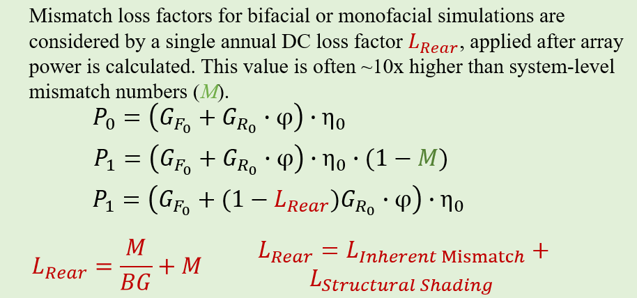
Ideally mismatch losses M should be calculated for the whole year, and then the mismatch loss factor to apply to Grear “Lrear” required by due diligence softwares can be calculated:
In this journal we will explore calculating mismatch loss M for a reduced set of hours. A procedure similar to that in Tutorial 3 will be used to generate various hourly irradiance measurements in the results folder, which the mismatch.py module will load and analyze. Analysis is done with PVMismatch, so this must be installed.
STEPS:#
1. Run an hourly simulation
2. Do mismatch analysis on the results.
1. Run an hourly simulation#
This will generate the results over which we will perform the mismatch analysis. Here we are doing only 1 day to make this faster.
[2]:
import bifacial_radiance
import os
from pathlib import Path

testfolder = str(Path().resolve().parent.parent / 'bifacial_radiance' / 'TEMP'/ 'Tutorial_08')
if not os.path.exists(testfolder):
    os.makedirs(testfolder)

simulationName = 'tutorial_8'
moduletype = "PVmodule"
albedo = 0.25
lat = 37.5
lon = -77.6

# Scene variables
nMods = 20
nRows = 7
hub_height = 1.5 # meters
gcr = 0.33

# Traking parameters
cumulativesky = False
limit_angle = 60
angledelta = 0.01
backtrack = True

#makeModule parameters
x = 1
y = 2
xgap = 0.01
zgap = 0.05
ygap = 0.0  # numpanels=1 anyways so it doesnt matter anyway
numpanels = 1
axisofrotationTorqueTube = True
diameter = 0.1
tubetype = 'Oct'
material = 'black'
tubeParams = {'diameter':diameter,
              'tubetype':tubetype,
              'material':material,
              'axisofrotation':axisofrotationTorqueTube,
              'visible':True}

# Analysis parmaeters
startdate = '11_06_08'       # Options: mm_dd, mm_dd_HH, mm_dd_HHMM, YYYY-mm-dd_HHMM
enddate = '11_06_10'
sensorsy = 12

demo = bifacial_radiance.RadianceObj(simulationName, path=testfolder)
demo.setGround(albedo)
epwfile = demo.getEPW(lat,lon)
metdata = demo.readWeatherFile(epwfile, starttime=startdate, endtime=enddate)
mymodule = demo.makeModule(name=moduletype, x=x, y=y, xgap=xgap,
                           ygap = ygap, zgap=zgap, numpanels=numpanels, tubeParams=tubeParams)
pitch = mymodule.sceney/gcr
sceneDict = {'pitch':pitch,'hub_height':hub_height, 'nMods': nMods, 'nRows': nRows}
demo.set1axis(limit_angle = limit_angle, backtrack = backtrack, gcr = gcr, cumulativesky = cumulativesky)
demo.gendaylit1axis()
demo.makeScene1axis(module=mymodule, sceneDict=sceneDict)
demo.makeOct1axis()
demo.analysis1axis(sensorsy = sensorsy);
path = F:\Documents\Python Scripts\bifacial_radiance\bifacial_radiance\TEMP\Tutorial_08
Loading albedo, 1 value(s), 0.250 avg
1 nonzero albedo values.
Getting weather file: USA_VA_Richmond.724010_TMY2.epw
 ... OK!
8760 line in WeatherFile. Assuming this is a standard hourly WeatherFile for the year for purposes of saving Gencumulativesky temporary weather files in EPW folder.
Coercing year to 2021
Filtering dates
Saving file EPWs\metdata_temp.csv, # points: 8760
Calculating Sun position for Metdata that is right-labeled  with a delta of -30 mins. i.e. 12 is 11:30 sunpos

Module Name: PVmodule
Module PVmodule updated in module.json
Pre-existing .rad file objects\PVmodule.rad will be overwritten

Creating ~3 skyfiles.
Created 3 skyfiles in /skies/

Making ~3 .rad files for gendaylit 1-axis workflow (this takes a minute..)
3 Radfiles created in /objects/

Making 3 octfiles in root directory.
Created 1axis_2021-11-06_0800.oct
Created 1axis_2021-11-06_0900.oct
Created 1axis_2021-11-06_1000.oct
Linescan in process: 1axis_2021-11-06_0800_Scene0_Row4_Module10_Front
Linescan in process: 1axis_2021-11-06_0800_Scene0_Row4_Module10_Back
Saved: results\irr_1axis_2021-11-06_0800_Scene0_Row4_Module10.csv
Index: 2021-11-06_0800. Wm2Front: 216.943925. Wm2Back: 6.079492166666667
Linescan in process: 1axis_2021-11-06_0900_Scene0_Row4_Module10_Front
Linescan in process: 1axis_2021-11-06_0900_Scene0_Row4_Module10_Back
Saved: results\irr_1axis_2021-11-06_0900_Scene0_Row4_Module10.csv
Index: 2021-11-06_0900. Wm2Front: 371.8801583333333. Wm2Back: 34.6894225
Linescan in process: 1axis_2021-11-06_1000_Scene0_Row4_Module10_Front
Linescan in process: 1axis_2021-11-06_1000_Scene0_Row4_Module10_Back
Saved: results\irr_1axis_2021-11-06_1000_Scene0_Row4_Module10.csv
Index: 2021-11-06_1000. Wm2Front: 335.72138333333334. Wm2Back: 41.0856625
2. Do mismatch analysis on the results#
There are various things that we need to know about the module at this stage.
Orientation: If it was simulated in portrait or landscape orientation.
Number of cells in the module: options right now are 72 or 96
Bifaciality factor: this is how well the rear of the module performs compared to the front of the module, and is a spec usually found in the datasheet.
Also, if the number of sampling points (sensorsy) from the result files does not match the number of cells along the panel orientation, downsampling or upsamplinb will be peformed. For this example, the module is in portrait mode (y > x), so there will be 12 cells along the collector width (numcellsy), and that’s why we set sensorsy = 12 during the analysis above.
These are the re-sampling options. To downsample, we suggest sensorsy >> numcellsy (for example, we’ve tested sensorsy = 100,120 and 200) - Downsamping by Center - Find the center points of all the sensors passed - Downsampling by Average - averages irradiances that fall on what would consist on the cell - Upsample
[3]:
resultfolder = os.path.join(testfolder, 'results')
writefiletitle = "Mismatch_Results.csv"

portraitorlandscape='portrait' # Options are 'portrait' or 'landscape'
bififactor=0.9 # Bifaciality factor DOES matter now, as the rear irradiance values will be multiplied by this factor.
numcells= 72# Options are 72 or 96 at the moment.
downsamplingmethod = 'byCenter' # Options are 'byCenter' or 'byAverage'.
analysisIrradianceandPowerMismatch(testfolder=resultfolder, writefiletitle=writefiletitle, portraitorlandscape=portraitorlandscape,
                                                              bififactor=bififactor, numcells=numcells)

print ("Your hourly mismatch values are now saved in the file above! :D")
6 files in the directory
Reads and calculates power output and mismatch for each file in the testfolder where all the bifacial_radiance irradiance results .csv are saved. First load each file, cleans it and resamples it to the numsensors set in this function, and then calculates irradiance mismatch and PVMismatch power output for averaged, minimum, or detailed irradiances on each cell for the cases of A) only 12 or 8 downsmaples values are considered (at the center of each cell), and B) 12 or 8 values are obtained from averaging all the irradiances falling in the area of the cell (No edges or inter-cell spacing are considered at this moment). Then it saves all the A and B irradiances, as well as the cleaned/resampled front and rear irradiances.
Ideally sensorsy in the read data is >> 12 to give results for the irradiance mismatch in the cell.
[5]:
def analysisIrradianceandPowerMismatch(testfolder, writefiletitle, portraitorlandscape, bififactor, numcells=72, downsamplingmethod='byCenter'):
    r'''
    Use this when sensorsy calculated with bifacial_radiance > cellsy


    Parameters
    ----------
    testfolder:   folder containing output .csv files for bifacial_radiance
    writefiletitle:   .csv title where the output results will be saved.
    portraitorlandscape: 'portrait' or 'landscape', for PVMismatch input
                      which defines the electrical interconnects inside the module.
    bififactor: bifaciality factor of the module. Max 1.0. ALL Rear irradiance values saved include the bifi-factor.
    downsampling method: 1 - 'byCenter' - 2 - 'byAverage'

    Example:

    # User information.
    import bifacial_radiance
    testfolder=r'C:\Users\sayala\Documents\HPC_Scratch\EUPVSEC\HPC Tracking Results\RICHMOND\Bifacial_Radiance Results\PVPMC_0\results'
    writefiletitle= r'C:\Users\sayala\Documents\HPC_Scratch\EUPVSEC\HPC Tracking Results\RICHMOND\Bifacial_Radiance Results\PVPMC_0\test_df.csv'
    sensorsy=100
    portraitorlandscape = 'portrait'
    analysis.analysisIrradianceandPowerMismatch(testfolder, writefiletitle, portraitorlandscape, bififactor=1.0, numcells=72)

    '''
    from bifacial_radiance import load
    import os, glob
    import pandas as pd

    # Default variables
    numpanels=1 # 1 at the moment, necessary for the cleaning routine.
    automatic=True

    #loadandclean
    # testfolder = r'C:\Users\sayala\Documents\HPC_Scratch\EUPVSEC\PinPV_Bifacial_Radiance_Runs\HPCResults\df4_FixedTilt\FixedTilt_Cairo_C_0.15\results'
    filelist = sorted(os.listdir(testfolder))
    #filelist = sorted(glob.glob(os.path.join('testfolder','*.csv')))
    print('{} files in the directory'.format(filelist.__len__()))

    # Check number of sensors on data.
    temp = load.read1Result(os.path.join(testfolder,filelist[0]))
    sensorsy = len(temp)

    # Setup PVMismatch parameters
    stdpl, cellsx, cellsy = _setupforPVMismatch(portraitorlandscape=portraitorlandscape, sensorsy=sensorsy, numcells=numcells)

    F=pd.DataFrame()
    B=pd.DataFrame()
    for z in range(0, filelist.__len__()):
            data=load.read1Result(os.path.join(testfolder,filelist[z]))
            [frontres, backres] = load.deepcleanResult(data, sensorsy=sensorsy, numpanels=numpanels, automatic=automatic)
            F[filelist[z]]=frontres
            B[filelist[z]]=backres

    B = B*bififactor
    # Downsample routines:
    if sensorsy > cellsy:
        if downsamplingmethod == 'byCenter':
            print("Sensors y > cellsy; Downsampling data by finding CellCenter method")
            F = _sensorsdownsampletocellbyCenter(F, cellsy)
            B = _sensorsdownsampletocellbyCenter(B, cellsy)
        elif downsamplingmethod == 'byAverage':
            print("Sensors y > cellsy; Downsampling data by Averaging data into Cells method")
            F = _sensorsdownsampletocellsbyAverage(F, cellsy)
            B = _sensorsdownsampletocellsbyAverage(B, cellsy)
        else:
            print ("Sensors y > cellsy for your module. Select a proper downsampling method ('byCenter', or 'byAverage')")
            return
    elif sensorsy < cellsy:
        print("Sensors y < cellsy; Upsampling data by Interpolation")
        F = _sensorupsampletocellsbyInterpolation(F, cellsy)
        B = _sensorupsampletocellsbyInterpolation(B, cellsy)
    elif sensorsy == cellsy:
        print ("Same number of sensorsy and cellsy for your module.")
        F = F
        B = B

    # Calculate POATs
    Poat = F+B

    # Define arrays to fill in:
    Pavg_all=[]; Pdet_all=[]
    Pavg_front_all=[]; Pdet_front_all=[]
    colkeys = F.keys()

    import pvmismatch

    if cellsx*cellsy == 72:
        cell_pos = pvmismatch.pvmismatch_lib.pvmodule.STD72
    elif cellsx*cellsy == 96:
        cell_pos = pvmismatch.pvmismatch_lib.pvmodule.STD96
    else:
        print("Error. Only 72 and 96 cells modules supported at the moment. Change numcells to either of this options!")
        return

    pvmod=pvmismatch.pvmismatch_lib.pvmodule.PVmodule(cell_pos=cell_pos)
    pvsys = pvmismatch.pvsystem.PVsystem(numberStrs=1, numberMods=1, pvmods=pvmod)


    # Calculate powers for each hour:
    for i in range(0,len(colkeys)):
        Pavg, Pdet = calculatePVMismatch(pvsys = pvsys, stdpl=stdpl, cellsx=cellsx, cellsy=cellsy, Gpoat=list(Poat[colkeys[i]]/1000))
        Pavg_front, Pdet_front = calculatePVMismatch(pvsys = pvsys, stdpl = stdpl, cellsx = cellsx, cellsy = cellsy, Gpoat= list(F[colkeys[i]]/1000))
        Pavg_all.append(Pavg)
        Pdet_all.append(Pdet)
        Pavg_front_all.append(Pavg_front)
        Pdet_front_all.append(Pdet_front)

    ## Rename Rows and save dataframe and outputs.
    F.index='FrontIrradiance_cell_'+F.index.astype(str)
    B.index='BackIrradiance_cell_'+B.index.astype(str)
    Poat.index='POAT_Irradiance_cell_'+Poat.index.astype(str)

    # Statistics Calculatoins
    dfst=pd.DataFrame()
    dfst['MAD/G_Total'] = mad_fn(Poat)
    dfst['Front_MAD/G_Total'] = mad_fn(F)
    dfst['MAD/G_Total**2'] = dfst['MAD/G_Total']**2
    dfst['Front_MAD/G_Total**2'] = dfst['Front_MAD/G_Total']**2
    dfst['poat'] = Poat.mean()
    dfst['gfront'] = F.mean()
    dfst['grear'] = B.mean()
    dfst['bifi_ratio'] =  dfst['grear']/dfst['gfront']
    dfst['stdev'] = Poat.std()/ dfst['poat']
    dfst.index=Poat.columns.astype(str)

    # Power Calculations/Saving
    Pout=pd.DataFrame()
    Pout['Pavg']=Pavg_all
    Pout['Pdet']=Pdet_all
    Pout['Front_Pavg']=Pavg_front_all
    Pout['Front_Pdet']=Pdet_front_all
    Pout['Mismatch_rel'] = 100-(Pout['Pdet']*100/Pout['Pavg'])
    Pout['Front_Mismatch_rel'] = 100-(Pout['Front_Pdet']*100/Pout['Front_Pavg'])
    Pout.index=Poat.columns.astype(str)

    ## Save CSV as one long row
    df_all = pd.concat([Pout, dfst, Poat.T, F.T, B.T], axis=1)
    df_all.to_csv(writefiletitle)
    print("Saved Results to ", writefiletitle)
[7]:
def _setupforPVMismatch(portraitorlandscape, sensorsy, numcells=72):
    r''' Sets values for calling PVMismatch, for ladscape or portrait modes and

    Example:
    stdpl, cellsx, cellsy = _setupforPVMismatch(portraitorlandscape='portrait', sensorsy=100):
    '''

    import numpy as np

        # cell placement for 'portrait'.
    if numcells == 72:
        stdpl=np.array([[0, 23,     24,     47,     48,     71],
        [1, 22,     25,     46,     49,     70],
        [2, 21,     26,     45,     50,     69],
        [3, 20,     27,     44,     51,     68],
        [4, 19,     28,     43,     52,     67],
        [5, 18,     29,     42,     53,     66],
        [6, 17,     30,     41,     54,     65],
        [7, 16,     31,     40,     55,     64],
        [8, 15,     32,     39,     56,     63],
        [9, 14,     33,     38,     57,     62],
        [10,        13,     34,     37,     58,     61],
        [11,        12,     35,     36,     59,     60]])

    elif numcells == 96:
        stdpl=np.array([[0, 23,     24,     47,     48,     71,     72,     95],
            [1,     22,     25,     46,     49,     70,     73,     94],
            [2,     21,     26,     45,     50,     69,     74,     93],
            [3,     20,     27,     44,     51,     68,     75,     92],
            [4,     19,     28,     43,     52,     67,     76,     91],
            [5,     18,     29,     42,     53,     66,     77,     90],
            [6,     17,     30,     41,     54,     65,     78,     89],
            [7,     16,     31,     40,     55,     64,     79,     88],
            [8,     15,     32,     39,     56,     63,     80,     87],
            [9,     14,     33,     38,     57,     62,     81,     86],
            [10,    13,     34,     37,     58,     61,     82,     85],
            [11,    12,     35,     36,     59,     60,     83,     84]])
    else:
        print("Error. Only 72 and 96 cells modules supported at the moment. Change numcells to either of this options!")
        return

    if portraitorlandscape == 'landscape':
        stdpl = stdpl.transpose()
    elif portraitorlandscape != 'portrait':
        print("Error. portraitorlandscape variable must either be 'landscape' or 'portrait'")
        return

    cellsx = len(stdpl[1]); cellsy = len(stdpl)

    return stdpl, cellsx, cellsy
We hope to add more content to this journal for next release so check back! Particularly how to use the Mad_fn to make the mismatch calculation faster, as per the proceedings and publication above!