[1]:
# This information helps with debugging and getting support :)
import sys, platform
import pandas as pd
import bifacial_radiance as br
print("Working on a ", platform.system(), platform.release())
print("Python version ", sys.version)
print("Pandas version ", pd.__version__)
print("bifacial_radiance version ", br.__version__)
Working on a  Windows 10
Python version  3.11.8 | packaged by conda-forge | (main, Feb 16 2024, 20:40:50) [MSC v.1937 64 bit (AMD64)]
Pandas version  2.2.3
bifacial_radiance version  0.5.0b2.dev4+gedb973d.d20250924
7 - Multiple Scene Objects#
This journal shows how to:
Create multiple scene objects in the same scene.
Analyze multiple scene objects in the same scene
Add a marker to find the origin (0,0) on a scene (for sanity-checks/visualization).
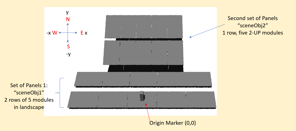
A scene Object is defined as an array of modules, with whatever parameters you want to give it. In this case, we are modeling one array of 2 rows of 5 modules in landscape, and one array of 1 row of 5 modules in 2-UP, portrait configuration, as the image below:
Steps:#
Generating the setups
Generating the firt scene object
Generating the second scene object.
Add a Marker at the Origin (coordinates 0,0) for help with visualization
Combine all scene Objects into one OCT file & Visualize
Analysis for Each sceneObject
1. Generating the Setups#
[2]:
import os
import numpy as np
import pandas as pd
from pathlib import Path

testfolder = str(Path().resolve().parent.parent / 'bifacial_radiance' / 'TEMP' / 'Tutorial_07')
if not os.path.exists(testfolder):
    os.makedirs(testfolder)

print ("Your simulation will be stored in %s" % testfolder)

from bifacial_radiance import RadianceObj, AnalysisObj
Your simulation will be stored in C:\Users\cdeline\Documents\Python Scripts\Bifacial_Radiance\bifacial_radiance\TEMP\Tutorial_07
A. Generating the first scene object#
This is a standard fixed-tilt setup for one hour. Gencumsky could be used too for the whole year.
The key here is that we are setting in sceneDict the variable appendRadfile to true.
[3]:
demo = RadianceObj("tutorial_7", path = testfolder)
demo.setGround(0.62)
epwfile = demo.getEPW(lat = 37.5, lon = -77.6)
metdata = demo.readWeatherFile(epwfile, coerce_year=2001)
fullYear = True
timestamp = metdata.datetime.index(pd.to_datetime('2001-06-17 13:0:0 -5'))  # Noon, June 17th
demo.gendaylit(timestamp)
module_type = 'test-moduleA'
mymodule = demo.makeModule(name=module_type,y=1,x=1.7)
sceneDict = {'tilt':10,'pitch':1.5,'clearance_height':0.2,'azimuth':180, 'nMods': 5, 'nRows': 2}
sceneObj1 = demo.makeScene(mymodule, sceneDict)
path = C:\Users\cdeline\Documents\Python Scripts\Bifacial_Radiance\bifacial_radiance\TEMP\Tutorial_07
Loading albedo, 1 value(s), 0.620 avg
1 nonzero albedo values.
Getting weather file: USA_VA_Richmond.724010_TMY2.epw
 ... OK!
8760 line in WeatherFile. Assuming this is a standard hourly WeatherFile for the year for purposes of saving Gencumulativesky temporary weather files in EPW folder.
Coercing year to 2001
Saving file EPWs\metdata_temp.csv, # points: 8760
Calculating Sun position for Metdata that is right-labeled  with a delta of -30 mins. i.e. 12 is 11:30 sunpos

Module Name: test-moduleA
Module test-moduleA updated in module.json
Pre-existing .rad file objects\test-moduleA.rad will be overwritten
Checking values after Scene for the scene Object created
[4]:
print ("SceneObj1 modulefile: %s" % sceneObj1.modulefile)
print ("SceneObj1 SceneFile: %s" %sceneObj1.radfiles)
print ("SceneObj1 GCR: %s" % round(sceneObj1.gcr,2))
print ("FileLists: \n %s" % demo.getfilelist())
SceneObj1 modulefile: objects\test-moduleA.rad
SceneObj1 SceneFile: ['objects\\test-moduleA_C_0.20_rtr_1.50_tilt_10_5modsx2rows_origin0,0.rad']
SceneObj1 GCR: 0.67
FileLists:
 ['materials\\ground.rad', 'skies\\sky2_37.5_-77.33_2001-06-17_1300.rad', 'objects\\test-moduleA_C_0.20_rtr_1.50_tilt_10_5modsx2rows_origin0,0.rad']
B. Generating the second scene object.#
Creating a different Scene. Same Module, different values. Notice we are passing a different originx and originy to displace the center of this new sceneObj to that location.
To make this work, we need to use append=True. Otherwise the second scene will overwrite the first.
[5]:
sceneDict2 = {'tilt':30,'pitch':5,'clearance_height':1,'azimuth':180,
              'nMods': 5, 'nRows': 1, 'originx': 0, 'originy': 3.5, 'appendRadfile':True}
module_type2='test-moduleB'
mymodule2 = demo.makeModule(name=module_type2,x=1,y=1.6, numpanels=2, ygap=0.15)
sceneObj2 = demo.makeScene(mymodule2, sceneDict2, append=True)

demo.sceneNames()
Module Name: test-moduleB
Module test-moduleB updated in module.json
Pre-existing .rad file objects\test-moduleB.rad will be overwritten

Additional scene Scene1 created! See list of names with RadianceObj.scenes and sceneNames
[5]:
['Scene0', 'Scene1']
[6]:
# Checking values for both scenes after creating new SceneObj
print ("SceneObj1 modulefile: %s" % sceneObj1.modulefile)
print ("SceneObj1 SceneFile: %s" %sceneObj1.radfiles)
print ("SceneObj1 GCR: %s" % round(sceneObj1.gcr,2))

print ("\nSceneObj2 modulefile: %s" % sceneObj2.modulefile)
print ("SceneObj2 SceneFile: %s" %sceneObj2.radfiles)
print ("SceneObj2 GCR: %s" % round(sceneObj2.gcr,2))

#getfilelist should have info for the rad file created by BOTH scene objects.
print ("NEW FileLists: \n %s" % demo.getfilelist())
SceneObj1 modulefile: objects\test-moduleA.rad
SceneObj1 SceneFile: ['objects\\test-moduleA_C_0.20_rtr_1.50_tilt_10_5modsx2rows_origin0,0.rad']
SceneObj1 GCR: 0.67

SceneObj2 modulefile: objects\test-moduleB.rad
SceneObj2 SceneFile: ['objects\\test-moduleB_C_1.00_rtr_5.00_tilt_30_5modsx1rows_origin0,3.5.rad']
SceneObj2 GCR: 0.67
NEW FileLists:
 ['materials\\ground.rad', 'skies\\sky2_37.5_-77.33_2001-06-17_1300.rad', 'objects\\test-moduleA_C_0.20_rtr_1.50_tilt_10_5modsx2rows_origin0,0.rad', 'objects\\test-moduleB_C_1.00_rtr_5.00_tilt_30_5modsx1rows_origin0,3.5.rad']
2. Add a Marker at the Origin (coordinates 0,0) for help with visualization#
Creating a “markers” for the geometry is useful to orient one-self when doing sanity-checks (for example, marke where 0,0 is, or where 5,0 coordinate is).
Note that if you analyze the module that intersects with the marker, some of the sensors will be wrong. To perform valid analysis, do so without markers, as they are ‘real’ objects on your scene.
[7]:
# NOTE: offsetting translation by 0.1 so the center of the marker (with sides of 0.2) is at the desired coordinate.
name='Post1'
text='! genbox black originMarker 0.2 0.2 1 | xform -t -0.1 -0.1 0'
customRadfile = demo.makeCustomObject(name,text)
sceneObj1.appendtoScene(customObject=customRadfile)
Custom Object Name objects\Post1.rad
3. Combine all scene Objects into one OCT file & Visualize#
Marking this as its own steps because this is the step that joins our Scene Objects 1, 2 and the appended Post. Run makeOCT to make the scene with both scene objects AND the marker in it, the ground and the skies.
[8]:
octfile = demo.makeOct(demo.getfilelist())
Created tutorial_7.oct
At this point you should be able to go into a command window (cmd.exe) and check the geometry. Example:
rvu -vf views:nbsphinx-math:front.vp -e .01 -pe 0.3 -vp 1 -7.5 12 tutorial_7.oct#
[9]:
## Comment the ! line below to run rvu from the Jupyter notebook instead of your terminal.
## Simulation will stop until you close the rvu window

#!rvu -vf views\front.vp -e .01 -pe 0.3 -vp 1 -7.5 12 tutorial_7.oct
It should look something like this:
4. Analysis for Each sceneObject#
a sceneDict is saved for each scene. When calling the Analysis, you should reference the scene object you want.
[9]:
sceneObj1.sceneDict
[9]:
{'tilt': 10,
 'pitch': 1.5,
 'clearance_height': 0.2,
 'azimuth': 180,
 'nMods': 5,
 'nRows': 2,
 'axis_tilt': 0,
 'originx': 0,
 'originy': 0}
[10]:
sceneObj2.sceneDict
[10]:
{'tilt': 30,
 'pitch': 5,
 'clearance_height': 1,
 'azimuth': 180,
 'nMods': 5,
 'nRows': 1,
 'originx': 0,
 'originy': 3.5,
 'appendRadfile': True,
 'axis_tilt': 0}
[11]:
analysis = AnalysisObj(octfile, demo.basename)
frontscan, backscan = analysis.moduleAnalysis(sceneObj1)
frontdict, backdict = analysis.analysis(octfile, "FirstObj", frontscan, backscan)  # compare the back vs front irradiance
print('Annual bifacial ratio First Set of Panels: %0.3f ' %( np.mean(analysis.Wm2Back) / np.mean(analysis.Wm2Front)) )
Linescan in process: FirstObj_Row1_Module3_Front
Linescan in process: FirstObj_Row1_Module3_Back
Saved: results\irr_FirstObj_Row1_Module3.csv
Annual bifacial ratio First Set of Panels: 0.129
Let’s do a Sanity check for first object: Since we didn’t pass any desired module, it should grab the center module of the center row (rounding down). For 2 rows and 5 modules, that is row 1, module 3 ~ indexed at 0, a2.0.a0.PVmodule…..””
[12]:
print (frontdict['x'])
print ("")
print (frontdict['y'])
print ("")
print (frontdict['mattype'])
[0. 0. 0. 0. 0. 0. 0. 0. 0.]

[-0.3982  -0.2998  -0.2012  -0.1028  -0.00415  0.0945   0.1926   0.2913
  0.39   ]

['a2.0.a0.test-moduleA.6457' 'a2.0.a0.test-moduleA.6457'
 'a2.0.a0.test-moduleA.6457' 'a2.0.a0.test-moduleA.6457'
 'a2.0.a0.test-moduleA.6457' 'a2.0.a0.test-moduleA.6457'
 'a2.0.a0.test-moduleA.6457' 'a2.0.a0.test-moduleA.6457'
 'a2.0.a0.test-moduleA.6457']
Let’s analyze a module in sceneobject 2 now. Remember we can specify which module/row we want. We only have one row in this Object though.
[13]:
analysis2 = AnalysisObj(octfile, demo.basename)
modWanted = 4
rowWanted = 1
sensorsy=4
frontscan, backscan = analysis2.moduleAnalysis(sceneObj2, modWanted = modWanted, rowWanted = rowWanted, sensorsy=sensorsy)
frontdict2, backdict2 = analysis2.analysis(octfile, "SecondObj", frontscan, backscan)
print('Annual bifacial ratio Second Set of Panels: %0.3f ' %( np.mean(analysis2.Wm2Back) / np.mean(analysis2.Wm2Front)) )
Linescan in process: SecondObj_Row1_Module4_Front
Linescan in process: SecondObj_Row1_Module4_Back
Saved: results\irr_SecondObj_Row1_Module4.csv
Annual bifacial ratio Second Set of Panels: 0.294
[14]:
analysis2 = AnalysisObj(octfile, demo.basename)
modWanted = 4
rowWanted = 1
sensorsy=4
frontscan, backscan = analysis2.moduleAnalysis(sceneObj2, modWanted = modWanted, rowWanted = rowWanted, sensorsy=sensorsy)
frontdict2, backdict2 = analysis2.analysis(octfile, "SecondObj", frontscan, backscan)
print('Annual bifacial ratio Second Set of Panels: %0.3f ' %( np.mean(analysis2.Wm2Back) / np.mean(analysis2.Wm2Front)) )
Linescan in process: SecondObj_Row1_Module4_Front
Linescan in process: SecondObj_Row1_Module4_Back
Saved: results\irr_SecondObj_Row1_Module4.csv
Annual bifacial ratio Second Set of Panels: 0.293
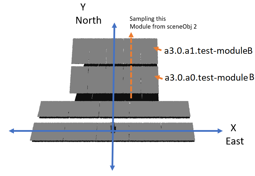
Sanity check for first object. Since we didn’t pass any desired module, it should grab the center module of the center row (rounding down). For 1 rows, that is row 0, module 4 ~ indexed at 0, a3.0.a0.Longi… and a3.0.a1.Longi since it is a 2-UP system.
[14]:
print ("x coordinate points:" , frontdict2['x'])
print ("")
print ("y coordinate points:", frontdict2['y'])
print ("")
print ("Elements intersected at each point: ", frontdict2['mattype'])
x coordinate points: [1.01 1.01 1.01 1.01]

y coordinate points: [2.617 3.197 3.777 4.36 ]

Elements intersected at each point:  ['a3.0.a0.test-moduleB.6457' 'a3.0.a0.test-moduleB.6457'
 'a3.0.a1.test-moduleB.6457' 'a3.0.a1.test-moduleB.6457']
Visualizing the coordinates and module analyzed with an image: