
[1]:
# This information helps with debugging and getting support :)
import sys, platform
import pandas as pd
import bifacial_radiance as br
print("Working on a ", platform.system(), platform.release())
print("Python version ", sys.version)
print("Pandas version ", pd.__version__)
print("bifacial_radiance version ", br.__version__)
Working on a  Windows 10
Python version  3.11.7 | packaged by Anaconda, Inc. | (main, Dec 15 2023, 18:05:47) [MSC v.1916 64 bit (AMD64)]
Pandas version  2.1.4
bifacial_radiance version  0+untagged.1553.g23d2640.dirty
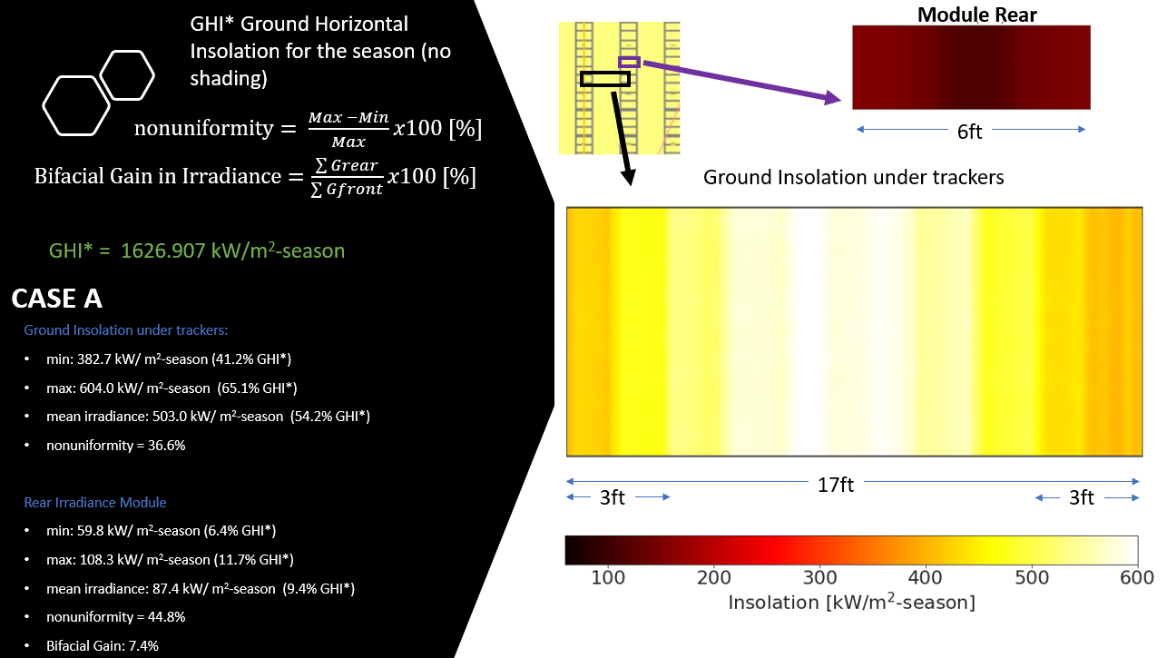
17 - AgriPV - Jack Solar Site Modeling#
Modeling Jack Solar AgriPV site in Longmonth CO, for crop season May September. The site has two configurations:
Configuration A:
Under 6 ft panels : 1.8288m
Hub height: 6 ft : 1.8288m
Configuration B:
8 ft panels : 2.4384m
Hub height 8 ft : 2.4384m
Other general parameters:
Module Size: 3ft x 6ft (portrait mode)
Row-to-row spacing: 17 ft –> 5.1816
Torquetube: square, diam 15 cm, zgap = 0
Albedo = green grass
Steps in this Journal:#
Load Bifacial Radiance and other essential packages
Define all the system variables
Build Scene for a pretty Image
More details#
There are three methods to perform the following analyzis:
Hourly with Fixed tilt, getTrackerAngle to update tilt of tracker
Hourly with gendaylit1axis using the tracking dictionary
Cumulatively with gencumsky1axis
The analysis itself is performed with the HPC with method A, and results are compared to GHI (equations below). The code below shows how to build the geometry and view it for accuracy, as well as evaluate monthly GHI, as well as how to model it with gencumsky1axis which is more suited for non-hpc environments.
1. Load Bifacial Radiance and other essential packages#
[1]:
import bifacial_radiance
import numpy as np
import os # this operative system to do the relative-path testfolder for this example.
import pprint    # We will be pretty-printing the trackerdictionary throughout to show its structure.
from pathlib import Path
import pandas as pd
2. Define all the system variables#
[2]:
testfolder = str(Path().resolve().parent.parent / 'bifacial_radiance' / 'Tutorial_17')
if not os.path.exists(testfolder):
    os.makedirs(testfolder)

timestamp = 4020 # Noon, June 17th.
simulationName = 'tutorial_17'    # Optionally adding a simulation name when defning RadianceObj

#Location
lat = 40.1217  # Given for the project site at Colorado
lon = -105.1310  # Given for the project site at Colorado

# MakeModule Parameters
moduletype='test-module'
numpanels = 1  # This site have 1 module in Y-direction
x = 1
y = 2
#xgap = 0.15 # Leaving 15 centimeters between modules on x direction
#ygap = 0.10 # Leaving 10 centimeters between modules on y direction
zgap = 0 # no gap to torquetube.
sensorsy = 6  # this will give 6 sensors per module in y-direction
sensorsx = 3   # this will give 3 sensors per module in x-direction

torquetube = True
axisofrotationTorqueTube = True
diameter = 0.15  # 15 cm diameter for the torquetube
tubetype = 'square'    # Put the right keyword upon reading the document
material = 'black'   # Torque tube of this material (0% reflectivity)

# Scene variables
nMods = 20
nRows = 7
hub_height = 1.8 # meters
pitch = 5.1816 # meters      # Pitch is the known parameter
albedo = 0.2  #'Grass'     # ground albedo
gcr = y/pitch

cumulativesky = False
limit_angle = 60 # tracker rotation limit angle
angledelta = 0.01 # we will be doing hourly simulation, we want the angle to be as close to real tracking as possible.
backtrack = True
[3]:
test_folder_fmt = 'Hour_{}'
3. Build Scene for a pretty Image#
[6]:
idx = 272

test_folderinner = os.path.join(testfolder, test_folder_fmt.format(f'{idx:04}'))
if not os.path.exists(test_folderinner):
    os.makedirs(test_folderinner)

rad_obj = bifacial_radiance.RadianceObj(simulationName,path = test_folderinner)  # Create a RadianceObj 'object'
rad_obj.setGround(albedo)
epwfile = rad_obj.getEPW(lat,lon)
metdata = rad_obj.readWeatherFile(epwfile, label='center', coerce_year=2021)
solpos = rad_obj.metdata.solpos.iloc[idx]
zen = float(solpos.zenith)
azm = float(solpos.azimuth) - 180
dni = rad_obj.metdata.dni[idx]
dhi = rad_obj.metdata.dhi[idx]
rad_obj.gendaylit(idx)
# rad_obj.gendaylit2manual(dni, dhi, 90 - zen, azm)
#print(rad_obj.metdata.datetime[idx])
tilt = round(rad_obj.getSingleTimestampTrackerAngle(metdata, timeindex=idx, gcr=gcr, limit_angle=65),1)
sceneDict = {'pitch': pitch, 'tilt': tilt, 'azimuth': 90, 'hub_height':hub_height, 'nMods':nMods, 'nRows': nRows}
scene = rad_obj.makeScene(module=moduletype,sceneDict=sceneDict)
octfile = rad_obj.makeOct()
path = C:\Users\mprillim\sam_dev\bifacial_radiance\bifacial_radiance\Tutorial_17\Hour_0272
Loading albedo, 1 value(s), 0.200 avg
1 nonzero albedo values.
Getting weather file: USA_CO_Boulder-Broomfield-Jefferson.County.AP.724699_TMY3.epw
 ... OK!
8760 line in WeatherFile. Assuming this is a standard hourly WeatherFile for the year for purposes of saving Gencumulativesky temporary weather files in EPW folder.
Coercing year to 2021
Saving file EPWs\metdata_temp.csv, # points: 8760
Calculating Sun position for center labeled data, at exact timestamp in input Weather File
Created tutorial_17.oct
The scene generated can be viewed by navigating on the terminal to the testfolder and typing
rvu -vf views:nbsphinx-math:front.vp -e .0265652 -vp 2 -21 2.5 -vd 0 1 0 tutorial_17.oct
OR Comment the ! line below to run rvu from the Jupyter notebook instead of your terminal.
[7]:
## Comment the ! line below to run rvu from the Jupyter notebook instead of your terminal.
## Simulation will stop until you close the rvu window

#!rvu -vf views\front.vp -e .0265652 -vp 2 -21 2.5 -vd 0 1 0 tutorial_17.oct
GHI Calculations#
From Weather File#
[8]:
# BOULDER
# Simple method where I know the index where the month starts and collect the monthly values this way.

# In 8760 TMY, this were the indexes:
starts = [2881, 3626, 4346, 5090, 5835]
ends = [3621, 4341, 5085, 5829, 6550]

starts = [metdata.datetime.index(pd.to_datetime('2021-05-01 6:0:0 -7')),
          metdata.datetime.index(pd.to_datetime('2021-06-01 6:0:0 -7')),
          metdata.datetime.index(pd.to_datetime('2021-07-01 6:0:0 -7')),
          metdata.datetime.index(pd.to_datetime('2021-08-01 6:0:0 -7')),
          metdata.datetime.index(pd.to_datetime('2021-09-01 6:0:0 -7'))]

ends = [metdata.datetime.index(pd.to_datetime('2021-05-31 18:0:0 -7')),
          metdata.datetime.index(pd.to_datetime('2021-06-30 18:0:0 -7')),
          metdata.datetime.index(pd.to_datetime('2021-07-31 18:0:0 -7')),
          metdata.datetime.index(pd.to_datetime('2021-08-31 18:0:0 -7')),
          metdata.datetime.index(pd.to_datetime('2021-09-30 18:0:0 -7'))]

ghi_Boulder = []
for ii in range(0, len(starts)):
    start = starts[ii]
    end = ends[ii]
    ghi_Boulder.append(metdata.ghi[start:end].sum())
print(" GHI Boulder Monthly May to September Wh/m2:", ghi_Boulder)
GHI Boulder Monthly May to September Wh/m2: [196632, 206257, 201029, 176973, 146532]
With raytrace#
[9]:
simulationName = 'EMPTYFIELD_MAY'
starttime = pd.to_datetime('2021-05-01 6:0:0')
endtime = pd.to_datetime('2021-05-31 18:0:0')
rad_obj = bifacial_radiance.RadianceObj(simulationName)
rad_obj.setGround(albedo)
metdata = rad_obj.readWeatherFile(epwfile, label='center', coerce_year=2021, starttime=starttime, endtime=endtime)
rad_obj.genCumSky()
#print(rad_obj.metdata.datetime[idx])
sceneDict = {'pitch': pitch, 'tilt': 0, 'azimuth': 90, 'hub_height':-0.2, 'nMods':1, 'nRows': 1}
scene = rad_obj.makeScene(module=moduletype,sceneDict=sceneDict)
octfile = rad_obj.makeOct()
analysis = bifacial_radiance.AnalysisObj()
frontscan, backscan = analysis.moduleAnalysis(scene, sensorsy=1)
frontscan['zstart'] = 0.5
frontdict, backdict = analysis.analysis(octfile = octfile, name='FIELDTotal', frontscan=frontscan, backscan=backscan)
print("FIELD TOTAL MAY:", analysis.Wm2Front[0])
path = C:\Users\mprillim\sam_dev\bifacial_radiance\bifacial_radiance\Tutorial_17\Hour_0272
Loading albedo, 1 value(s), 0.200 avg
1 nonzero albedo values.
8760 line in WeatherFile. Assuming this is a standard hourly WeatherFile for the year for purposes of saving Gencumulativesky temporary weather files in EPW folder.
Coercing year to 2021
Filtering dates
Saving file EPWs\metdata_temp.csv, # points: 8760
Calculating Sun position for center labeled data, at exact timestamp in input Weather File
Loaded  EPWs\metdata_temp.csv
message: There were 461 sun up hours in this climate file
Total Ibh/Lbh: 0.000000
Created EMPTYFIELD_MAY.oct
Linescan in process: FIELDTotal_Front
Linescan in process: FIELDTotal_Back
Saved: results\irr_FIELDTotal.csv
FIELD TOTAL MAY: 194047.0