
[1]:
# This information helps with debugging and getting support :)
import sys, platform
import pandas as pd
import bifacial_radiance as br
print("Working on a ", platform.system(), platform.release())
print("Python version ", sys.version)
print("Pandas version ", pd.__version__)
print("bifacial_radiance version ", br.__version__)
Working on a  Windows 10
Python version  3.9.12 (main, Apr  4 2022, 05:22:27) [MSC v.1916 64 bit (AMD64)]
Pandas version  1.4.2
bifacial_radiance version  0.4.4.dev26+ge667a7c
3 - Single Axis Tracking Hourly#
Example demonstrating the use of doing hourly smiulations with Radiance gendaylit for 1-axis tracking. This is a medium level example because it also explores a couple subtopics:
Subtopics:
The structure of the tracker dictionary “trackerDict”.
How to calculate GCR
How to make a cell-level module
Various methods to use the trackerdictionary for analysis.
Doing full year simulations with gendaylit:
Performing the simulation hour by hour requires either a good computer or some patience, since there are ~4000 daylight-hours in the year. With a 32GB RAM, Windows 10 i7-8700 CPU @ 3.2GHz with 6 cores this takes 1 day. The code also allows for multiple cores or HPC use – there is documentation/examples inside the software at the moment, but that is an advanced topic. The procedure can be broken into shorter steps for one day or a single timestamp simulation which is exemplified below.
Steps:
Load bifacial_radiance
Define all your system variables
Create Radiance Object, Set Albedo and Weather
Make Module: Cell Level Module Example
Calculate GCR
Set Tracking Angles
Generate the Sky
Make Scene 1axis
Make Oct and AnalyzE 1 HOUR
Make Oct and Analye Range of Hours
Make Oct and Analyze All Tracking Dictionary
And finally: Condensed Version: All Tracking Dictionary
1. Load bifacial_radiance#
Pay attention: different importing method:
So far we’ve used “from bifacial_radiance import *” to import all the bifacial_radiance files into our working space in jupyter. For this journal we will do a “import bifacial_radiance” . This method of importing requires a different call for some functions as you’ll see below. For example, instead of calling demo = RadianceObj(path = testfolder) as on Tutorial 2, in this case we will neeed to do demo = bifacial_radiance.RadianceObj(path = testfolder).
[2]:
import bifacial_radiance
import numpy as np
import os # this operative system to do teh relative-path testfolder for this example.
import pprint    # We will be pretty-printing the trackerdictionary throughout to show its structure.
from pathlib import Path
2. Define all your system variables#
Just like in the condensed version show at the end of Tutorial 2, for this tutorial we will be starting all of our system variables from the beginning of the jupyter journal, instead than throughout the different cells (for the most part)
[3]:
testfolder = Path().resolve().parent.parent / 'bifacial_radiance' / 'TEMP' / 'Tutorial_03'
if not os.path.exists(testfolder):
    os.makedirs(testfolder)


simulationName = 'tutorial_03'    # For adding a simulation name when defning RadianceObj. This is optional.
moduletype = 'test-module'    # We will define the parameters for this below in Step 4.
albedo = "litesoil"      # this is one of the options on ground.rad
lat = 37.5
lon = -77.6

# Scene variables
nMods = 20
nRows = 7
hub_height = 2.3 # meters
pitch = 10 # meters      # We will be using pitch instead of GCR for this example.

# Traking parameters
cumulativesky = False
limit_angle = 45 # tracker rotation limit angle
angledelta = 0.01 # we will be doing hourly simulation, we want the angle to be as close to real tracking as possible.
backtrack = True

#makeModule parameters
# x and y will be defined later on Step 4 for this tutorial!!
xgap = 0.01
ygap = 0.10
zgap = 0.05
numpanels = 2
axisofrotation = True  #  the scene will rotate around the torque tube, and not the middle of the bottom surface of the module
diameter = 0.1
tubetype = 'Oct'    # This will make an octagonal torque tube.
material = 'black'   # Torque tube of this material (0% reflectivity)
3. Create Radiance Object, Set Albedo and Weather#
Same steps as previous two tutorials, so condensing it into one step. You hopefully have this down by now! :)
Notice that we are doing bifacial_radiance.RadianceObj because we change the import method for this example!
We now constrain the days of our analysis in the readWeatherFile import step. For this example we are doing just two days in January. Format has to be a ‘MM_DD’ or ‘YYYY-MM-DD_HHMM’
[4]:
demo = bifacial_radiance.RadianceObj(simulationName, path = str(testfolder))  # Adding a simulation name. This is optional.
demo.setGround(albedo)
epwfile = demo.getEPW(lat=lat, lon=lon)

starttime = '01_13';  endtime = '01_14'
metdata = demo.readWeatherFile(weatherFile=epwfile, starttime=starttime, endtime=endtime)
path = C:\Users\cdeline\Documents\Python Scripts\Bifacial_Radiance\bifacial_radiance\TEMP\Tutorial_03
Loading albedo, 1 value(s), 0.213 avg
1 nonzero albedo values.
Getting weather file: USA_VA_Richmond.724010_TMY2.epw
 ... OK!
8760 line in WeatherFile. Assuming this is a standard hourly WeatherFile for the year for purposes of saving Gencumulativesky temporary weather files in EPW folder.
Coercing year to 2021
Filtering dates
Saving file EPWs\metdata_temp.csv, # points: 8760
Calculating Sun position for Metdata that is right-labeled  with a delta of -30 mins. i.e. 12 is 11:30 sunpos
4. Make Module: Cell Level Module Example#
Instead of doing a opaque, flat single-surface module, in this tutorial we will create a module made up by cells. We can define variuos parameters to make a cell-level module, such as cell size and spacing between cells. To do this, we will pass a dicitonary with the needed parameters to makeModule, as shown below.
NOTE: in v0.4.0 some keywords and methods for doing a CellModule and Torquetube simulation were changed.
Since we are making a cell-level module, the dimensions for x and y of the module will be calculated by the software – dummy values can be initially passed just to get started, but these values are overwritten by addCellModule()
[5]:
numcellsx = 6
numcellsy = 12
xcell = 0.156
ycell = 0.156
xcellgap = 0.02
ycellgap = 0.02


mymodule = demo.makeModule(name=moduletype,  x=1, y=1, xgap=xgap, ygap=ygap,
                           zgap=zgap, numpanels=numpanels)
mymodule.addTorquetube(diameter=diameter, material=material,
                       axisofrotation=axisofrotation, tubetype=tubetype)
mymodule.addCellModule(numcellsx=numcellsx, numcellsy=numcellsy,
                       xcell=xcell, ycell=ycell, xcellgap=xcellgap, ycellgap=ycellgap)

print(f'New module created. x={mymodule.x}m,  y={mymodule.y}m')
print(f'Cell-module parameters: {mymodule.cellModule}')
Module Name: test-module
Module test-module updated in module.json
Pre-existing .rad file objects\test-module.rad will be overwritten

Module test-module updated in module.json
Pre-existing .rad file objects\test-module.rad will be overwritten

Module was shifted by 0.078 in X to avoid sensors on air
This is a Cell-Level detailed module with Packaging Factor of 0.81
Module test-module updated in module.json
Pre-existing .rad file objects\test-module.rad will be overwritten

New module created. x=1.036m,  y=2.092m
Cell-module parameters: {'numcellsx': 6, 'numcellsy': 12, 'xcell': 0.156, 'ycell': 0.156, 'xcellgap': 0.02, 'ycellgap': 0.02, 'centerJB': None}
5. Calculate GCR#
In this example we passed the parameter “pitch”. Pitch is the spacing between rows (for example, between hub-posts) in a field. To calculate Ground Coverage Ratio (GCR), we must relate the pitch to the collector-width by:
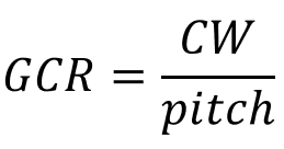
The collector width for our system must consider the number of panels and the y-gap:

Collector Width gets saved in your module parameters (and later on your scene and trackerdict) as “sceney”. You can calculate your collector width with the equation, or you can use this method to know your GCR:
[6]:
# For more options on makemodule, see the help description of the function.
# Details about the module are stored in the new ModuleObj
CW = mymodule.sceney
gcr = CW / pitch
print ("The GCR is :", gcr)
print(f"\nModuleObj data keys: {mymodule.keys}")
The GCR is : 0.4284

ModuleObj data keys: ['x', 'y', 'z', 'modulematerial', 'scenex', 'sceney', 'scenez', 'numpanels', 'bifi', 'text', 'modulefile', 'glass', 'glassEdge', 'offsetfromaxis', 'xgap', 'ygap', 'zgap']
6. Set Tracking Angles#
This function will read the weather file, and based on the sun position it will calculate the angle the tracker should be at for each hour. It will create metdata files for each of the tracker angles considered.
For doing hourly simulations, remember to set cumulativesky = False here!
[7]:
trackerdict = demo.set1axis(metdata=metdata, limit_angle=limit_angle, backtrack=backtrack,
                            gcr=gcr, cumulativesky=False)
[8]:
print ("Trackerdict created by set1axis: %s " % (len(demo.trackerdict)))
Trackerdict created by set1axis: 20
set1axis initializes the trackerdictionary Trackerdict. Trackerdict contains all hours selected from the weatherfile as keys. For example: trackerdict[‘2021-01-13_1200’]. It is a return variable on many of the 1axis functions, but it is also stored inside of your Radiance Obj (i.e. demo.trackerdict). In this journal we are storing it as a variable to mute the option (otherwise it prints the returned trackerdict contents every time)
[9]:
pprint.pprint(trackerdict['2021-01-13_1200'])
{'dhi': np.int64(200),
 'dni': np.int64(97),
 'ghi': np.int64(249),
 'surf_azm': 90.0,
 'surf_tilt': 21.2,
 'temp_air': np.float64(6.5),
 'theta': -21.2,
 'wind_speed': np.float64(3.9)}
All of the following functions add up elements to trackerdictionary to keep track (ba-dum tupzz) of the Scene and simulation parameters. In advanced journals we will explore the inner structure of trackerdict. For now, just now it exists :)
7. Generate the Sky#
We will create skies for each hour we want to model with the function gendaylit1axis.
For this example we are doing just two days in January. The ability to limit the time using gendaylit1axis is deprecated. Use readWeatherFile instead.
[10]:
trackerdict = demo.gendaylit1axis()
Creating ~20 skyfiles.
Created 20 skyfiles in /skies/
Since we passed startdate and enddate to gendaylit, it will prune our trackerdict to only the desired days. Let’s explore our trackerdict:
[11]:
trackerkeys = sorted(trackerdict.keys())
print ("Trackerdict option of hours are: ", trackerkeys)
print ("")
print ("Contents of trackerdict for sample hour:")
pprint.pprint(trackerdict[trackerkeys[0]])
Trackerdict option of hours are:  ['2021-01-13_0800', '2021-01-13_0900', '2021-01-13_1000', '2021-01-13_1100', '2021-01-13_1200', '2021-01-13_1300', '2021-01-13_1400', '2021-01-13_1500', '2021-01-13_1600', '2021-01-13_1700', '2021-01-14_0800', '2021-01-14_0900', '2021-01-14_1000', '2021-01-14_1100', '2021-01-14_1200', '2021-01-14_1300', '2021-01-14_1400', '2021-01-14_1500', '2021-01-14_1600', '2021-01-14_1700']

Contents of trackerdict for sample hour:
{'dhi': np.int64(22),
 'dni': np.int64(13),
 'ghi': np.int64(23),
 'skyfile': 'skies\\sky2_37.5_-77.33_2021-01-13_0800.rad',
 'surf_azm': 90.0,
 'surf_tilt': 3.74,
 'temp_air': np.float64(0.2),
 'theta': -3.74,
 'wind_speed': np.float64(2.6)}
8. Make Scene 1axis#
We can use gcr or pitch fo our scene dictionary.
[12]:
sceneDict = {'pitch': pitch,'hub_height':hub_height, 'nMods':nMods, 'nRows': nRows}

# making the different scenes for the 1-axis tracking for the dates in trackerdict2.
trackerdict = demo.makeScene1axis(trackerdict=trackerdict, module=mymodule, sceneDict=sceneDict)
Making ~20 .rad files for gendaylit 1-axis workflow (this takes a minute..)
20 Radfiles created in /objects/
The scene parameteres are now stored in the trackerdict. To view them and to access them:
[13]:
pprint.pprint(trackerdict[trackerkeys[0]])
{'dhi': np.int64(22),
 'dni': np.int64(13),
 'ghi': np.int64(23),
 'scenes': [<class 'bifacial_radiance.main.SceneObj'> : {'gcr': np.float64(0.4284), 'hpc': False, 'module': <class 'bifacial_radiance.module.ModuleObj'> : {'x': np.float64(1.036), 'y': np.float64(2.092), 'z': 0.02, 'modulematerial': 'black', 'scenex': np.float64(1.046), 'sceney': np.float64(4.284), 'scenez': np.float64(0.1), 'numpanels': 2, 'bifi': 1, 'text': '! genbox black cellPVmodule 0.156 0.156 0.02 | xform -t -0.44 -2.142 0.1 -a 6 -t 0.176 0 0 -a 12 -t 0 0.176 0 -a 2 -t 0 2.192 0\r\n! genbox black octtube1a 1.046 0.04142135623730951 0.1 | xform -t -0.523 -0.020711 -0.05\r\n! genbox black octtube1b 1.046 0.04142135623730951 0.1 | xform -t -0.445 -0.020711 -0.05 -rx 45 -t 0 0 0\r\n! genbox black octtube1c 1.046 0.04142135623730951 0.1 | xform -t -0.445 -0.020710678118654756 -0.05 -rx 90 -t 0 0 0\r\n! genbox black octtube1d 1.046 0.04142135623730951 0.1 | xform -t -0.445 -0.020710678118654756 -0.05 -rx 135 -t 0 0 0 ', 'modulefile': 'objects\\test-module.rad', 'glass': False, 'glassEdge': 0.01, 'offsetfromaxis': np.float64(0.1), 'xgap': 0.01, 'ygap': 0.1, 'zgap': 0.05}, 'modulefile': 'objects\\test-module.rad', 'name': 'Scene0', 'radfiles': 'objects\\1axis2021-01-13_0800__C_2.17_rtr_10.00_tilt_4_20modsx7rows_origin0,0.rad', 'sceneDict': {'pitch': 10, 'nMods': 20, 'nRows': 7, 'tilt': 3.74, 'clearance_height': np.float64(2.166802445305938), 'azimuth': 90.0, 'modulez': 0.02, 'axis_tilt': 0, 'originx': 0, 'originy': 0, 'hub_height': np.float64(2.3)}, 'text': '!xform -rx 3.74 -t 0 0 2.3 -a 20 -t 1.046 0 0 -a 7 -t 0 10 0 -i 1 -t -9.414 -30.0 0 -rz 90.0 -t 0 0 0 "objects\\test-module.rad"'}],
 'skyfile': 'skies\\sky2_37.5_-77.33_2021-01-13_0800.rad',
 'surf_azm': 90.0,
 'surf_tilt': 3.74,
 'temp_air': np.float64(0.2),
 'theta': -3.74,
 'wind_speed': np.float64(2.6)}
[15]:
pprint.pprint(demo.trackerdict[trackerkeys[5]]['scene'][0].__dict__)
{'gcr': np.float64(0.4284),
 'hpc': False,
 'module': <class 'bifacial_radiance.module.ModuleObj'> : {'x': np.float64(1.036), 'y': np.float64(2.092), 'z': 0.02, 'modulematerial': 'black', 'scenex': np.float64(1.046), 'sceney': np.float64(4.284), 'scenez': np.float64(0.1), 'numpanels': 2, 'bifi': 1, 'text': '! genbox black cellPVmodule 0.156 0.156 0.02 | xform -t -0.44 -2.142 0.1 -a 6 -t 0.176 0 0 -a 12 -t 0 0.176 0 -a 2 -t 0 2.192 0\r\n! genbox black octtube1a 1.046 0.04142135623730951 0.1 | xform -t -0.523 -0.020711 -0.05\r\n! genbox black octtube1b 1.046 0.04142135623730951 0.1 | xform -t -0.445 -0.020711 -0.05 -rx 45 -t 0 0 0\r\n! genbox black octtube1c 1.046 0.04142135623730951 0.1 | xform -t -0.445 -0.020710678118654756 -0.05 -rx 90 -t 0 0 0\r\n! genbox black octtube1d 1.046 0.04142135623730951 0.1 | xform -t -0.445 -0.020710678118654756 -0.05 -rx 135 -t 0 0 0 ', 'modulefile': 'objects\\test-module.rad', 'glass': False, 'glassEdge': 0.01, 'offsetfromaxis': np.float64(0.1), 'xgap': 0.01, 'ygap': 0.1, 'zgap': 0.05},
 'modulefile': 'objects\\test-module.rad',
 'name': 'Scene0',
 'radfiles': 'objects\\1axis2021-01-13_1300__C_2.11_rtr_10.00_tilt_-5_20modsx7rows_origin0,0.rad',
 'sceneDict': {'axis_tilt': 0,
               'azimuth': 90.0,
               'clearance_height': np.float64(2.111024390776987),
               'hub_height': np.float64(2.3),
               'modulez': 0.02,
               'nMods': 20,
               'nRows': 7,
               'originx': 0,
               'originy': 0,
               'pitch': 10,
               'tilt': -5.31},
 'text': '!xform -rx -5.31 -t 0 0 2.3 -a 20 -t 1.046 0 0 -a 7 -t 0 10 0 -i 1 '
         '-t -9.414 -30.0 0 -rz 90.0 -t 0 0 0 "objects\\test-module.rad"'}
9. Make Oct and Analyze#
A. Make Oct and Analyze 1Hour#
There are various options now to analyze the trackerdict hours we have defined. We will start by doing just one hour, because it’s the fastest. Make sure to select an hour that exists in your trackerdict!
Options of hours:
[16]:
pprint.pprint(trackerkeys)
['2021-01-13_0800',
 '2021-01-13_0900',
 '2021-01-13_1000',
 '2021-01-13_1100',
 '2021-01-13_1200',
 '2021-01-13_1300',
 '2021-01-13_1400',
 '2021-01-13_1500',
 '2021-01-13_1600',
 '2021-01-13_1700',
 '2021-01-14_0800',
 '2021-01-14_0900',
 '2021-01-14_1000',
 '2021-01-14_1100',
 '2021-01-14_1200',
 '2021-01-14_1300',
 '2021-01-14_1400',
 '2021-01-14_1500',
 '2021-01-14_1600',
 '2021-01-14_1700']
[16]:
demo.makeOct1axis(singleindex='2021-01-13_0800')
results = demo.analysis1axis(singleindex='2021-01-13_0800')
print('\n\nHourly bifi gain: {:0.3}'.format(sum(sum(demo.results.Wm2Back)) / sum(sum(demo.results.Wm2Front))))
Making 1 octfiles in root directory.
Created 1axis_2021-01-13_0800.oct
Linescan in process: 1axis_2021-01-13_0800_Scene0_Row4_Module10_Front
Linescan in process: 1axis_2021-01-13_0800_Scene0_Row4_Module10_Back
Saved: results\irr_1axis_2021-01-13_0800_Scene0_Row4_Module10.csv
Index: 2021-01-13_0800. Wm2Front: 23.62973037037037. Wm2Back: 2.8466184074074072


Hourly bifi gain: 0.125
The trackerdict now contains information about the octfile, as well as the Analysis Object results
[17]:
print ("\n Contents of trackerdict for sample hour after analysis1axis: ")
pprint.pprint(trackerdict[trackerkeys[0]])
 Contents of trackerdict for sample hour after analysis1axis:
{'AnalysisObj': [<class 'bifacial_radiance.main.AnalysisObj'> : {'Back/FrontRatio': [0.125, 0.123, 0.12, 0.118, 0.342, 0.114, 0.117, 0.118, 0.119], 'Wm2Back': [2.944, 2.899, 2.833, 2.786, 2.991, 2.694, 2.765, 2.804, 2.831], 'Wm2Front': [23.6, 23.602, 23.604, 23.605, 8.742, 23.691, 23.696, 23.702, 23.74], 'backRatio': [0.125, 0.123, 0.12, 0.118, 0.342, 0.114, 0.117, 0.118, 0.119], 'hpc': False, 'mattype': array(['a9.3.a2.2.0.cellPVmodule.6457', 'a9.3.a2.4.0.cellPVmodule.6457',
       'a9.3.a2.7.0.cellPVmodule.6457', 'a9.3.a2.9.0.cellPVmodule.6457',
       'a9.3.octtube1a.6457', 'a9.3.a2.2.1.cellPVmodule.6457',
       'a9.3.a2.4.1.cellPVmodule.6457', 'a9.3.a2.7.1.cellPVmodule.6457',
       'a9.3.a2.9.1.cellPVmodule.6457'], dtype=object), 'modWanted': 10, 'name': '1axis_2021-01-13_0800_Scene0', 'octfile': '1axis_2021-01-13_0800.oct', 'power_data': None, 'rearMat': array(['a9.3.a2.2.0.cellPVmodule.2310', 'a9.3.a2.4.0.cellPVmodule.2310',
       'a9.3.a2.7.0.cellPVmodule.2310', 'a9.3.a2.9.0.cellPVmodule.2310',
       'sky', 'a9.3.a2.2.1.cellPVmodule.2310',
       'a9.3.a2.4.1.cellPVmodule.2310', 'a9.3.a2.7.1.cellPVmodule.2310',
       'a9.3.a2.9.1.cellPVmodule.2310'], dtype=object), 'rearX': [1.716, 1.288, 0.861, 0.434, 0.006, -0.421, -0.849, -1.276, -1.704], 'rearY': [0.0, 0.0, 0.0, 0.0, 0.0, 0.0, 0.0, 0.0, 0.0], 'rearZ': [2.283, 2.31, 2.34, 2.367, 2.395, 2.422, 2.451, 2.479, 2.506], 'rowWanted': 4, 'sceneNum': 0, 'x': [1.718, 1.29, 0.863, 0.436, 0.008, -0.419, -0.847, -1.274, -1.702], 'y': [0.0, 0.0, 0.0, 0.0, 0.0, 0.0, 0.0, 0.0, 0.0], 'z': [2.312, 2.34, 2.37, 2.396, 2.424, 2.453, 2.48, 2.508, 2.535]},
                 <class 'bifacial_radiance.main.AnalysisObj'> : {'Back/FrontRatio': [0.124, 0.122, 0.12, 0.118, 0.133, 0.114, 0.117, 0.118, 0.119], 'Wm2Back': [2.946, 2.896, 2.844, 2.803, 2.991, 2.716, 2.791, 2.803, 2.829], 'Wm2Front': [23.785, 23.781, 23.777, 23.77, 22.482, 23.769, 23.769, 23.768, 23.768], 'backRatio': [0.124, 0.122, 0.12, 0.118, 0.133, 0.114, 0.117, 0.118, 0.119], 'hpc': False, 'mattype': array(['a9.3.a2.2.0.cellPVmodule.6457', 'a9.3.a2.4.0.cellPVmodule.6457',
       'a9.3.a2.7.0.cellPVmodule.6457', 'a9.3.a2.9.0.cellPVmodule.6457',
       'a9.3.octtube1a.6457', 'a9.3.a2.2.1.cellPVmodule.6457',
       'a9.3.a2.4.1.cellPVmodule.6457', 'a9.3.a2.7.1.cellPVmodule.6457',
       'a9.3.a2.9.1.cellPVmodule.6457'], dtype=object), 'modWanted': 10, 'name': '1axis_2021-01-13_0800_Scene0', 'octfile': '1axis_2021-01-13_0800.oct', 'power_data': None, 'rearMat': array(['a9.3.a2.2.0.cellPVmodule.2310', 'a9.3.a2.4.0.cellPVmodule.2310',
       'a9.3.a2.7.0.cellPVmodule.2310', 'a9.3.a2.9.0.cellPVmodule.2310',
       'sky', 'a9.3.a2.2.1.cellPVmodule.2310',
       'a9.3.a2.4.1.cellPVmodule.2310', 'a9.3.a2.7.1.cellPVmodule.2310',
       'a9.3.a2.9.1.cellPVmodule.2310'], dtype=object), 'rearX': [1.716, 1.288, 0.861, 0.434, 0.006, -0.421, -0.849, -1.276, -1.704], 'rearY': [0.0, 0.0, 0.0, 0.0, 0.0, 0.0, 0.0, 0.0, 0.0], 'rearZ': [2.283, 2.31, 2.34, 2.367, 2.395, 2.422, 2.451, 2.479, 2.506], 'rowWanted': 4, 'sceneNum': 0, 'x': [1.718, 1.29, 0.863, 0.436, 0.008, -0.419, -0.847, -1.274, -1.702], 'y': [0.0, 0.0, 0.0, 0.0, 0.0, 0.0, 0.0, 0.0, 0.0], 'z': [2.312, 2.34, 2.37, 2.396, 2.424, 2.453, 2.48, 2.508, 2.535]}],
 'dhi': np.int64(22),
 'dni': np.int64(13),
 'ghi': np.int64(23),
 'octfile': '1axis_2021-01-13_0800.oct',
 'scenes': [<class 'bifacial_radiance.main.SceneObj'> : {'gcr': np.float64(0.4284), 'hpc': False, 'module': <class 'bifacial_radiance.module.ModuleObj'> : {'x': np.float64(1.036), 'y': np.float64(2.092), 'z': 0.02, 'modulematerial': 'black', 'scenex': np.float64(1.046), 'sceney': np.float64(4.284), 'scenez': np.float64(0.1), 'numpanels': 2, 'bifi': 1, 'text': '! genbox black cellPVmodule 0.156 0.156 0.02 | xform -t -0.44 -2.142 0.1 -a 6 -t 0.176 0 0 -a 12 -t 0 0.176 0 -a 2 -t 0 2.192 0\r\n! genbox black octtube1a 1.046 0.04142135623730951 0.1 | xform -t -0.523 -0.020711 -0.05\r\n! genbox black octtube1b 1.046 0.04142135623730951 0.1 | xform -t -0.445 -0.020711 -0.05 -rx 45 -t 0 0 0\r\n! genbox black octtube1c 1.046 0.04142135623730951 0.1 | xform -t -0.445 -0.020710678118654756 -0.05 -rx 90 -t 0 0 0\r\n! genbox black octtube1d 1.046 0.04142135623730951 0.1 | xform -t -0.445 -0.020710678118654756 -0.05 -rx 135 -t 0 0 0 ', 'modulefile': 'objects\\test-module.rad', 'glass': False, 'glassEdge': 0.01, 'offsetfromaxis': np.float64(0.1), 'xgap': 0.01, 'ygap': 0.1, 'zgap': 0.05}, 'modulefile': 'objects\\test-module.rad', 'name': 'Scene0', 'radfiles': 'objects\\1axis2021-01-13_0800__C_2.17_rtr_10.00_tilt_4_20modsx7rows_origin0,0.rad', 'sceneDict': {'pitch': 10, 'nMods': 20, 'nRows': 7, 'tilt': 3.74, 'azimuth': 90.0, 'modulez': 0.02, 'axis_tilt': 0, 'originx': 0, 'originy': 0, 'hub_height': np.float64(2.3)}, 'text': '!xform -rx 3.74 -t 0 0 2.3 -a 20 -t 1.046 0 0 -a 7 -t 0 10 0 -i 1 -t -9.414 -30.0 0 -rz 90.0 -t 0 0 0 "objects\\test-module.rad"'}],
 'skyfile': 'skies\\sky2_37.5_-77.33_2021-01-13_0800.rad',
 'surf_azm': 90.0,
 'surf_tilt': 3.74,
 'temp_air': np.float64(0.2),
 'theta': -3.74,
 'wind_speed': np.float64(2.6)}
[18]:
pprint.pprint(trackerdict[trackerkeys[0]]['AnalysisObj'])
[<class 'bifacial_radiance.main.AnalysisObj'> : {'Back/FrontRatio': [0.125, 0.123, 0.12, 0.118, 0.342, 0.114, 0.117, 0.118, 0.119], 'Wm2Back': [2.944, 2.899, 2.833, 2.786, 2.991, 2.694, 2.765, 2.804, 2.831], 'Wm2Front': [23.6, 23.602, 23.604, 23.605, 8.742, 23.691, 23.696, 23.702, 23.74], 'backRatio': [0.125, 0.123, 0.12, 0.118, 0.342, 0.114, 0.117, 0.118, 0.119], 'hpc': False, 'mattype': array(['a9.3.a2.2.0.cellPVmodule.6457', 'a9.3.a2.4.0.cellPVmodule.6457',
       'a9.3.a2.7.0.cellPVmodule.6457', 'a9.3.a2.9.0.cellPVmodule.6457',
       'a9.3.octtube1a.6457', 'a9.3.a2.2.1.cellPVmodule.6457',
       'a9.3.a2.4.1.cellPVmodule.6457', 'a9.3.a2.7.1.cellPVmodule.6457',
       'a9.3.a2.9.1.cellPVmodule.6457'], dtype=object), 'modWanted': 10, 'name': '1axis_2021-01-13_0800_Scene0', 'octfile': '1axis_2021-01-13_0800.oct', 'power_data': None, 'rearMat': array(['a9.3.a2.2.0.cellPVmodule.2310', 'a9.3.a2.4.0.cellPVmodule.2310',
       'a9.3.a2.7.0.cellPVmodule.2310', 'a9.3.a2.9.0.cellPVmodule.2310',
       'sky', 'a9.3.a2.2.1.cellPVmodule.2310',
       'a9.3.a2.4.1.cellPVmodule.2310', 'a9.3.a2.7.1.cellPVmodule.2310',
       'a9.3.a2.9.1.cellPVmodule.2310'], dtype=object), 'rearX': [1.716, 1.288, 0.861, 0.434, 0.006, -0.421, -0.849, -1.276, -1.704], 'rearY': [0.0, 0.0, 0.0, 0.0, 0.0, 0.0, 0.0, 0.0, 0.0], 'rearZ': [2.283, 2.31, 2.34, 2.367, 2.395, 2.422, 2.451, 2.479, 2.506], 'rowWanted': 4, 'sceneNum': 0, 'x': [1.718, 1.29, 0.863, 0.436, 0.008, -0.419, -0.847, -1.274, -1.702], 'y': [0.0, 0.0, 0.0, 0.0, 0.0, 0.0, 0.0, 0.0, 0.0], 'z': [2.312, 2.34, 2.37, 2.396, 2.424, 2.453, 2.48, 2.508, 2.535]},
 <class 'bifacial_radiance.main.AnalysisObj'> : {'Back/FrontRatio': [0.124, 0.122, 0.12, 0.118, 0.133, 0.114, 0.117, 0.118, 0.119], 'Wm2Back': [2.946, 2.896, 2.844, 2.803, 2.991, 2.716, 2.791, 2.803, 2.829], 'Wm2Front': [23.785, 23.781, 23.777, 23.77, 22.482, 23.769, 23.769, 23.768, 23.768], 'backRatio': [0.124, 0.122, 0.12, 0.118, 0.133, 0.114, 0.117, 0.118, 0.119], 'hpc': False, 'mattype': array(['a9.3.a2.2.0.cellPVmodule.6457', 'a9.3.a2.4.0.cellPVmodule.6457',
       'a9.3.a2.7.0.cellPVmodule.6457', 'a9.3.a2.9.0.cellPVmodule.6457',
       'a9.3.octtube1a.6457', 'a9.3.a2.2.1.cellPVmodule.6457',
       'a9.3.a2.4.1.cellPVmodule.6457', 'a9.3.a2.7.1.cellPVmodule.6457',
       'a9.3.a2.9.1.cellPVmodule.6457'], dtype=object), 'modWanted': 10, 'name': '1axis_2021-01-13_0800_Scene0', 'octfile': '1axis_2021-01-13_0800.oct', 'power_data': None, 'rearMat': array(['a9.3.a2.2.0.cellPVmodule.2310', 'a9.3.a2.4.0.cellPVmodule.2310',
       'a9.3.a2.7.0.cellPVmodule.2310', 'a9.3.a2.9.0.cellPVmodule.2310',
       'sky', 'a9.3.a2.2.1.cellPVmodule.2310',
       'a9.3.a2.4.1.cellPVmodule.2310', 'a9.3.a2.7.1.cellPVmodule.2310',
       'a9.3.a2.9.1.cellPVmodule.2310'], dtype=object), 'rearX': [1.716, 1.288, 0.861, 0.434, 0.006, -0.421, -0.849, -1.276, -1.704], 'rearY': [0.0, 0.0, 0.0, 0.0, 0.0, 0.0, 0.0, 0.0, 0.0], 'rearZ': [2.283, 2.31, 2.34, 2.367, 2.395, 2.422, 2.451, 2.479, 2.506], 'rowWanted': 4, 'sceneNum': 0, 'x': [1.718, 1.29, 0.863, 0.436, 0.008, -0.419, -0.847, -1.274, -1.702], 'y': [0.0, 0.0, 0.0, 0.0, 0.0, 0.0, 0.0, 0.0, 0.0], 'z': [2.312, 2.34, 2.37, 2.396, 2.424, 2.453, 2.48, 2.508, 2.535]}]
B. Make Oct and Analye Range of Hours#
You could do a list of indices following a similar procedure:
[19]:
for time in ['2021-01-13_0900','2021-01-13_1300']:
    demo.makeOct1axis(singleindex=time)
    results=demo.analysis1axis(singleindex=time)
print('Accumulated hourly bifi gain: {:0.3}'.format(sum(sum(demo.results.Wm2Back)) / sum(sum(demo.results.Wm2Front))))
Making 1 octfiles in root directory.
Created 1axis_2021-01-13_0900.oct
Linescan in process: 1axis_2021-01-13_0900_Scene0_Row4_Module10_Front
Linescan in process: 1axis_2021-01-13_0900_Scene0_Row4_Module10_Back
Saved: results\irr_1axis_2021-01-13_0900_Scene0_Row4_Module10.csv
Index: 2021-01-13_0900. Wm2Front: 90.91053000000001. Wm2Back: 7.274867259259259

Making 1 octfiles in root directory.
Created 1axis_2021-01-13_1300.oct
Linescan in process: 1axis_2021-01-13_1300_Scene0_Row4_Module10_Front
Linescan in process: 1axis_2021-01-13_1300_Scene0_Row4_Module10_Back
Saved: results\irr_1axis_2021-01-13_1300_Scene0_Row4_Module10.csv
Index: 2021-01-13_1300. Wm2Front: 218.4903. Wm2Back: 31.121771111111116
Accumulated hourly bifi gain: 0.124
Note that the bifacial gain printed above is for the accumulated irradiance between the hours modeled so far. Results are stored in demo.results for each module, row, scene and timestamp.
[20]:
demo.results
[20]:
| timestamp | name | modNum | rowNum | sceneNum | x | y | z | rearZ | mattype | rearMat | Wm2Front | Wm2Back | backRatio | rearX | rearY | surf_azm | surf_tilt | theta | |
|---|---|---|---|---|---|---|---|---|---|---|---|---|---|---|---|---|---|---|---|
| 0 | 2021-01-13_0800 | 1axis_2021-01-13_0800_Scene0 | 10 | 4 | 0 | [1.718, 1.29, 0.863, 0.4355, 0.007812, -0.419,... | [0.0, 0.0, 0.0, 0.0, 0.0, 0.0, 0.0, 0.0, 0.0] | [2.312, 2.34, 2.37, 2.396, 2.424, 2.453, 2.48,... | [2.283, 2.31, 2.34, 2.367, 2.395, 2.422, 2.451... | [a9.3.a2.2.0.cellPVmodule.6457, a9.3.a2.4.0.ce... | [a9.3.a2.2.0.cellPVmodule.2310, a9.3.a2.4.0.ce... | [23.600226666666668, 23.60168, 23.60356, 23.60... | [2.944065666666667, 2.8991749999999996, 2.8331... | [0.1247420614295754, 0.12283244953539171, 0.12... | [1.716, 1.288, 0.861, 0.4336, 0.00586, -0.421,... | [0.0, 0.0, 0.0, 0.0, 0.0, 0.0, 0.0, 0.0, 0.0] | 90.0 | 3.74 | -3.74 |
| 1 | 2021-01-13_0800 | 1axis_2021-01-13_0800_Scene0 | 10 | 4 | 0 | [1.718, 1.29, 0.863, 0.4355, 0.007812, -0.419,... | [0.0, 0.0, 0.0, 0.0, 0.0, 0.0, 0.0, 0.0, 0.0] | [2.312, 2.34, 2.37, 2.396, 2.424, 2.453, 2.48,... | [2.283, 2.31, 2.34, 2.367, 2.395, 2.422, 2.451... | [a9.3.a2.2.0.cellPVmodule.6457, a9.3.a2.4.0.ce... | [a9.3.a2.2.0.cellPVmodule.2310, a9.3.a2.4.0.ce... | [23.78451, 23.78058, 23.77708, 23.770213333333... | [2.9459510000000004, 2.895887333333333, 2.8438... | [0.12385485953422903, 0.12177018235682124, 0.1... | [1.716, 1.288, 0.861, 0.4336, 0.00586, -0.421,... | [0.0, 0.0, 0.0, 0.0, 0.0, 0.0, 0.0, 0.0, 0.0] | 90.0 | 3.74 | -3.74 |
| 2 | 2021-01-13_0900 | 1axis_2021-01-13_0900_Scene0 | 10 | 4 | 0 | [1.664, 1.258, 0.852, 0.4463, 0.04004, -0.3652... | [0.0, 0.0, 0.0, 0.0, 0.0, 0.0, 0.0, 0.0, 0.0] | [1.871, 2.008, 2.145, 2.281, 2.418, 2.555, 2.6... | [1.843, 1.9795, 2.117, 2.254, 2.39, 2.527, 2.6... | [a9.3.a2.2.0.cellPVmodule.6457, a9.3.a2.4.0.ce... | [a9.3.a2.2.0.cellPVmodule.2310, a9.3.a2.4.0.ce... | [95.69555666666668, 96.40040333333333, 98.3446... | [7.239717333333334, 7.025711333333334, 6.65101... | [0.0756528509019499, 0.07287976202006188, 0.06... | [1.654, 1.248, 0.8423, 0.4365, 0.03027, -0.375... | [0.0, 0.0, 0.0, 0.0, 0.0, 0.0, 0.0, 0.0, 0.0] | 90.0 | 18.64 | -18.64 |
| 3 | 2021-01-13_1300 | 1axis_2021-01-13_1300_Scene0 | 10 | 4 | 0 | [1.694, 1.268, 0.8413, 0.415, -0.01172, -0.438... | [0.0, 0.0, 0.0, 0.0, 0.0, 0.0, 0.0, 0.0, 0.0] | [2.584, 2.545, 2.504, 2.465, 2.426, 2.387, 2.3... | [2.553, 2.514, 2.473, 2.434, 2.395, 2.355, 2.3... | [a9.3.a2.2.0.cellPVmodule.6457, a9.3.a2.4.0.ce... | [a9.3.a2.2.0.cellPVmodule.2310, a9.3.a2.4.0.ce... | [218.81786666666667, 218.82646666666665, 218.8... | [27.896079999999998, 26.794673333333332, 25.55... | [0.12748480249874858, 0.12244657282510545, 0.1... | [1.697, 1.2705, 0.844, 0.418, -0.00879, -0.435... | [0.0, 0.0, 0.0, 0.0, 0.0, 0.0, 0.0, 0.0, 0.0] | 90.0 | -5.31 | 5.31 |
To print the specific bifacial gain for a specific hour, you can refer back to the trackerdict:
[21]:
trackerdict['2021-01-13_1300']['AnalysisObj'][0].results
[21]:
| name | modNum | rowNum | sceneNum | x | y | z | rearZ | mattype | rearMat | Wm2Front | Wm2Back | backRatio | rearX | rearY | |
|---|---|---|---|---|---|---|---|---|---|---|---|---|---|---|---|
| 0 | 1axis_2021-01-13_1300_Scene0 | 10 | 4 | 0 | [1.694, 1.268, 0.8413, 0.415, -0.01172, -0.438... | [0.0, 0.0, 0.0, 0.0, 0.0, 0.0, 0.0, 0.0, 0.0] | [2.584, 2.545, 2.504, 2.465, 2.426, 2.387, 2.3... | [2.553, 2.514, 2.473, 2.434, 2.395, 2.355, 2.3... | [a9.3.a2.2.0.cellPVmodule.6457, a9.3.a2.4.0.ce... | [a9.3.a2.2.0.cellPVmodule.2310, a9.3.a2.4.0.ce... | [218.81786666666667, 218.82646666666665, 218.8... | [27.896079999999998, 26.794673333333332, 25.55... | [0.12748480249874858, 0.12244657282510545, 0.1... | [1.697, 1.2705, 0.844, 0.418, -0.00879, -0.435... | [0.0, 0.0, 0.0, 0.0, 0.0, 0.0, 0.0, 0.0, 0.0] |
[49]:
sum(sum(trackerdict['2021-01-13_1300']['AnalysisObj'][0].results.Wm2Back)) / sum(sum(trackerdict['2021-01-13_1300']['AnalysisObj'][0].results.Wm2Front))
[49]:
np.float64(0.1422167846598289)
C. Make Oct and Analyze All Tracking Dictionary#
This takes considerably more time, depending on the number of entries on the trackerdictionary. If no starttime and endtime were specified on STEP readWeatherFile, this will run ALL of the hours in the year (~4000 hours).
[ ]:
demo.makeOct1axis()
results = demo.analysis1axis()
print('Accumulated hourly bifi gain for all the trackerdict: {:0.3}'.format(sum(sum(demo.results.Wm2Back)) / sum(sum(demo.results.Wm2Front))))
Remember you should clean your results first! This will have torquetube and sky results if performed this way so don’t trust this simplistic bifacial_gain examples.
Condensed Version: All Tracking Dictionary#
This is the summarized version to run gendaylit for each entry in the trackingdictionary.
[ ]:
import bifacial_radiance
import os

simulationName = 'Tutorial 3'
moduletype = 'Custom Cell-Level Module'
testfolder = os.path.abspath(r'..\..\bifacial_radiance\TEMP')
albedo = "litesoil"
lat = 37.5
lon = -77.6

# Scene variables
nMods = 20
nRows = 7
hub_height = 2.3 # meters
pitch = 10 # meters

# Traking parameters
cumulativesky = False
limit_angle = 45 # degrees
angledelta = 0.01 #
backtrack = True

#makeModule parameters
# x and y will do not need to be defined as they are calculated internally for cell-level modules
xgap = 0.01
ygap = 0.10
zgap = 0.05
numpanels = 2

cellModuleParams = {'numcellsx': 6,
'numcellsy': 12,
'xcell': 0.156,
'ycell': 0.156,
'xcellgap': 0.02,
'ycellgap': 0.02}


torquetube = True
axisofrotation = True  # the scene will rotate around the torque tube, and not the middle of the bottom surface of the module
diameter = 0.1
tubetype = 'Oct'    # This will make an octagonal torque tube.
material = 'black'   # Torque tube material (0% reflectivity)
tubeParams = {'diameter':diameter,
              'tubetype':tubetype,
              'material':material,
              'axisofrotation':axisofrotation}

startdate = '11_06'
enddate = '11_06'
demo = bifacial_radiance.RadianceObj(simulationName, path=testfolder)
demo.setGround(albedo)
epwfile = demo.getEPW(lat,lon)
metdata = demo.readWeatherFile(epwfile, starttime=startdate, endtime=enddate)
mymodule = bifacial_radiance.ModuleObj(name=moduletype, xgap=xgap, ygap=ygap,
                zgap=zgap, numpanels=numpanels, cellModule=cellModuleParams, tubeParams=tubeParams)
sceneDict = {'pitch':pitch, 'hub_height':hub_height, 'nMods': nMods, 'nRows':nRows}
demo.set1axis(limit_angle=limit_angle, backtrack=backtrack, gcr=gcr, cumulativesky=cumulativesky)
demo.gendaylit1axis()
demo.makeScene1axis(module=mymodule, sceneDict=sceneDict) #makeScene creates a .rad file with 20 modules per row, 7 rows.
demo.makeOct1axis()
demo.analysis1axis()