
[1]:
# This information helps with debugging and getting support :)
import sys, platform
import pandas as pd
import bifacial_radiance as br
import numpy as np
print("Working on a ", platform.system(), platform.release())
print("Python version ", sys.version)
print("Pandas version ", pd.__version__)
print("bifacial_radiance version ", br.__version__)
Working on a  Windows 10
Python version  3.11.8 | packaged by conda-forge | (main, Feb 16 2024, 20:40:50) [MSC v.1937 64 bit (AMD64)]
Pandas version  2.2.3
bifacial_radiance version  0.5.0b2.dev4+gedb973d.d20250924
5 - Bifacial Carports and Canopies#
This journal shows how to model a carport or canopy ~ a fixed structure, usually at a high clearance from the ground, with more than one bifacial solar module in the same inclined-plane to create a “shade” for the cars/people below.
We assume that bifacia_radiacne is already installed in yoru computer. This works for bifacial_radiance v.3 release.
These journal outlines 4 useful uses of bifacial_radiance and some tricks:
Creating the modules in the canopy/carport
Adding extra geometry for the pillars/posts supporting the carport/canopy
Sampling the rear irradiance with more resolution (more sensors)
and hacking the sensor position to obtain an irradiance map of rear-irradiance.
Adding an object to simulate a car with a specific reflectivity.
This is what we will create: 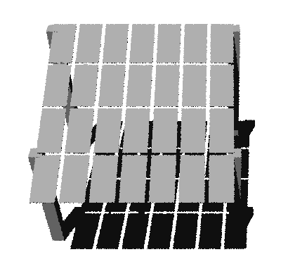
Steps:#
Setup of Variables through Making OCT Axis
Adding the pillars
Analysis of the collector width
Mapping the irradiance througout all the Carport
Adding a “Car”
1. Setup of Variables through Making OCT Axis#
We’ve done this before a couple times, no new stuff here.
The magic is that, for doing the carport we see in the figure, we are going to do a 4-up configuration of modules (numpanels), and we are going to repeat that 4-UP 7 times (nMods)
[3]:
from pathlib import Path
testfolder = str(Path().resolve().parent.parent / 'bifacial_radiance' / 'TEMP')

print ("Your simulation will be stored in %s" % testfolder)

simulationname = 'tutorial_5'

# MakeModule Parameters
moduletype='test-module'
numpanels = 4  # Carport will have 4 modules along the y direction (N-S since we are facing it to the south) .
x = 0.95
y = 1.95
xgap = 0.15 # Leaving 15 centimeters between modules on x direction
ygap = 0.10 # Leaving 10 centimeters between modules on y direction
zgap = 0 # no gap between modules and torquetube.
sensorsy = 10*numpanels  # this will give 70 sensors per module.

# Other default values:

# TorqueTube Parameters
torquetube = False

# SceneDict Parameters
gcr = 0.33   # We are only doing 1 row so this doesn't matter
albedo = 0.28  #'concrete'     # ground albedo
clearance_height = 4.3 # m
nMods = 7 # six modules length.
nRows = 1  # only 1 row

azimuth_ang=180 # Facing south
tilt =20 # tilt.


## Now let's run the example

demo = br.RadianceObj(simulationname,path = testfolder)
demo.setGround(albedo)
epwfile = demo.getEPW(40.0583,-74.4057) # NJ lat/lon 40.0583° N, 74.4057
metdata = demo.readWeatherFile(epwfile, coerce_year=2021)

timestamp = metdata.datetime.index(pd.to_datetime('2021-06-17 13:0:0 -5'))
demo.gendaylit(timestamp)  # Use this to simulate only one hour at a time.

mymodule=demo.makeModule(name=moduletype,x=x,y=y,numpanels = numpanels, xgap=xgap, ygap=ygap, torquetube=torquetube)

sceneDict = {'tilt':tilt,'pitch': round(gcr/mymodule.sceney,3),'clearance_height':clearance_height,'azimuth':azimuth_ang, 'module_type':moduletype, 'nMods': nMods, 'nRows': nRows}
scene = demo.makeScene(module=mymodule, sceneDict=sceneDict)
octfile = demo.makeOct(demo.getfilelist())
Your simulation will be stored in C:\Users\cdeline\Documents\Python Scripts\Bifacial_Radiance\bifacial_radiance\TEMP
path = C:\Users\cdeline\Documents\Python Scripts\Bifacial_Radiance\bifacial_radiance\TEMP
Loading albedo, 1 value(s), 0.280 avg
1 nonzero albedo values.
Getting weather file: USA_NJ_McGuire.AFB.724096_TMY3.epw
 ... OK!
8760 line in WeatherFile. Assuming this is a standard hourly WeatherFile for the year for purposes of saving Gencumulativesky temporary weather files in EPW folder.
Coercing year to 2021
Saving file EPWs\metdata_temp.csv, # points: 8760
Calculating Sun position for Metdata that is right-labeled  with a delta of -30 mins. i.e. 12 is 11:30 sunpos

Warning: boolean input `torquetube` passed into makeModule. Starting in v0.4.0 this boolean parameter is deprecated. Use module.addTorquetube() with `visible` parameter instead.

Module Name: test-module
Module test-module updated in module.json
Pre-existing .rad file objects\test-module.rad will be overwritten

Created tutorial_5.oct
If you view the Oct file at this point, you should see the array of 7 modules, with 4 modules each along the collector widt.
2. Adding the pillars#
We will add 4 pillars at roughly the back and front corners of the structure. Some of the code below is to calculate the positions of where the pillars will be at.
We are calculating the location with some math geometry
[4]:
xright= x*4
xleft=  -xright

y2nd = -(y*numpanels/2)*np.cos(tilt*np.pi/180) + (y)*np.cos(tilt*np.pi/180)
y6th=  -(y*numpanels/2)*np.cos(tilt*np.pi/180) + (y*numpanels)*np.cos(tilt*np.pi/180)
z2nd = (y*np.sin(tilt*np.pi/180))+clearance_height
z6th =  (y*numpanels)*np.sin(tilt*np.pi/180)+clearance_height

name='Post1'
text='! genbox black cuteBox 0.5 0.5 {} | xform -t -0.25 -0.25 0 -t {} {} 0'.format(z2nd, xleft, y2nd)
print (text)
customObject = demo.makeCustomObject(name,text)
scene.appendtoScene(customObject=customObject)

name='Post2'
text='! genbox black cuteBox 0.5 0.5 {} | xform -t -0.25 -0.25 0 -t {} {} 0'.format(z2nd, xright, y2nd)
customObject = demo.makeCustomObject(name,text)
scene.appendtoScene(customObject=customObject)

name='Post3'
text='! genbox black cuteBox 0.5 0.5 {} | xform -t -0.25 -0.25 0 -t {} {} 0'.format(z6th, xright, y6th)
customObject = demo.makeCustomObject(name,text)
scene.appendtoScene(customObject=customObject)

name='Post4'
text='! genbox black cuteBox 0.5 0.5 {} | xform -t -0.25 -0.25 0 -t {} {} 0'.format(z6th, xleft, y6th)
customObject = demo.makeCustomObject(name,text)
scene.appendtoScene(customObject=customObject)

octfile = demo.makeOct()  # makeOct combines all of the ground, sky and object files into a .oct file.
! genbox black cuteBox 0.5 0.5 4.966939279485054 | xform -t -0.25 -0.25 0 -t -3.8 -1.8324006105325215 0

Custom Object Name objects\Post1.rad

Custom Object Name objects\Post2.rad

Custom Object Name objects\Post3.rad

Custom Object Name objects\Post4.rad
Created tutorial_5.oct
View the geometry with the posts on :#
rvu -vf views:nbsphinx-math:`front`.vp -e .01 -pe 0.4 -vp 3.5 -20 22 tutorial_5.oct
-pe sets the exposure levels, and -vp sets the view point so the carport is centered (at least on my screen. you can play with the values). It should look like this:
The post should be coindient with the corners of the array on the high-end of the carport, and on the low end of the carport they should be between the lowest module and the next one. Cute!
[4]:
## Comment the ! line below to run rvu from the Jupyter notebook instead of your terminal.
## Simulation will stop until you close the rvu window

#!rvu -vf views\front.vp -e .01 -pe 0.4 -vp 3.5 -20 22 tutorial_5.oct
3. Analysis of the collector width#
Now let’s do some analysis along the slope of the modules. Each result file will contain irradiance for the 4 modules that make up the slope of the carport. You can select which “module” along the row you sample too.
We are also increasign the number of points sampled accross the collector width, with the variable sensorsy passed to moduleanalysis
[10]:
analysis = br.AnalysisObj(octfile, demo.name)
modWanted = 1
rowWanted = 1
frontscan, backscan = analysis.moduleAnalysis(scene, modWanted=modWanted, rowWanted=rowWanted, sensorsy=sensorsy)

analysis.analysis(octfile, simulationname+"Mod1", frontscan, backscan)
print('Annual bifacial ratio average:  %0.3f' %( sum(analysis.Wm2Back) / sum(analysis.Wm2Front) ) )
print("")
Linescan in process: tutorial_5Mod1_Row1_Module1_Front
Linescan in process: tutorial_5Mod1_Row1_Module1_Back
Saved: results\irr_tutorial_5Mod1_Row1_Module1.csv
Annual bifacial ratio average:  0.179
This is the module analysis and an image of the results file 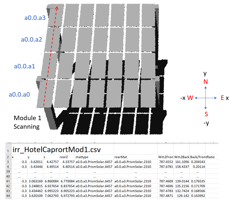
(Notice in the image above the module name we originally used in this tutorial was “Prism Solar” and not “test-module”. Otherwise your results should look the same.)
You can repeat the analysis for any other module in the row:
Notice we are passing a CUSTOM simulation name so the results are generated in separate csv files.
[7]:
modWanted = 2
rowWanted = 1
frontscan, backscan = analysis.moduleAnalysis(scene, modWanted=modWanted, rowWanted=rowWanted, sensorsy=sensorsy)

analysis.analysis(octfile, simulationname+"Mod2", frontscan, backscan)
print('Annual bifacial ratio average:  %0.3f' %( sum(analysis.Wm2Back) / sum(analysis.Wm2Front))  )


modWanted = 3
rowWanted = 1
frontscan, backscan = analysis.moduleAnalysis(scene, modWanted=modWanted, rowWanted=rowWanted, sensorsy=sensorsy)

analysis.analysis(octfile, simulationname+"Mod3", frontscan, backscan)
print('Annual bifacial ratio average:  %0.3f' %( sum(analysis.Wm2Back) / sum(analysis.Wm2Front) ) )
Linescan in process: tutorial_5Mod2_Row1_Module2_Front
Linescan in process: tutorial_5Mod2_Row1_Module2_Back
Saved: results\irr_tutorial_5Mod2_Row1_Module2.csv
Annual bifacial ratio average:  0.175
Linescan in process: tutorial_5Mod3_Row1_Module3_Front
Linescan in process: tutorial_5Mod3_Row1_Module3_Back
Saved: results\irr_tutorial_5Mod3_Row1_Module3.csv
Annual bifacial ratio average:  0.173
4. Mapping the irradiance througout all the Carport (“Hack” the sensors)#
You can “hack” the sensors starting locations to obtain an irradinace distribution map. This is easier when the modules are facing South, or East/West. Below is an example, you’ll have to repeat over all the modules/ all the surface area with as much resolution as you have patience to see edge-effects.
[8]:
# HACK Frontscan and Backscan
frontscan['xstart']=-1.2

analysis.analysis(octfile, simulationname+"Mod3_point2", frontscan, backscan)
print('Annual bifacial ratio average:  %0.3f' %( sum(analysis.Wm2Back)  / sum(analysis.Wm2Front) ) )
Linescan in process: tutorial_5Mod3_point2_Row1_Module3_Front
Linescan in process: tutorial_5Mod3_point2_Row1_Module3_Back
Saved: results\irr_tutorial_5Mod3_point2_Row1_Module3.csv
Annual bifacial ratio average:  0.173
The printed Annual bifacial ratio does not include cleaning of the sensors for the material. Some of the sensros might fall in the spacing between the modules (ygaps) or in the structures added, torquetubes, etc. For a real bifacial ratio gain, use the load and clean functions in load.py.
(This process might be automated in a future release TBD)
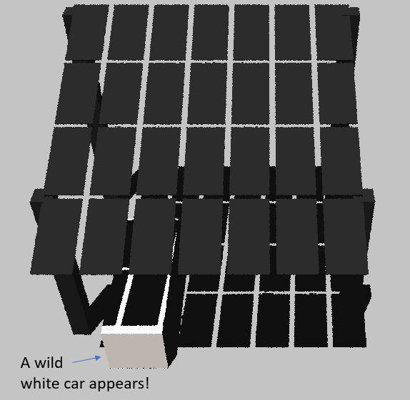
5. Adding a “Car”#
Add a surface (just like we added the pillars) with a specific reflectivity to represent a car. If you are doing hourly simulation you can compare how much the irradiance increases with and without the car, and if you keep track of your parking lot comings/goings this could make an interesting toy-problem: how much are your employees contributing to your rear irradiance production?
[9]:
name='Car_1'
carpositionx=-2
carpositiony=-1
text='! genbox white_EPDM HondaFit 1.6 4.5 1.5 | xform -t -0.8 -2.25 0 -t {} {} 0'.format(carpositionx, carpositiony)
customObject = demo.makeCustomObject(name,text)
scene.appendtoScene(customObject=customObject)

octfile = demo.makeOct(demo.getfilelist())  # run makeOct to combine the ground, sky and all new scene object files
Custom Object Name objects\Car_1.rad
Created tutorial_5.oct
Viewing with: ## rvu -vf views:nbsphinx-math:front.vp -e .01 -pe 0.019 -vp 1.5 -14 15 tutorial_5.oct
[10]:
## Comment the ! line below to run rvu from the Jupyter notebook instead of your terminal.
## Simulation will stop until you close the rvu window

!rvu -vf views\front.vp -e .01 -pe 0.019 -vp 1.5 -14 15 tutorial_5.oct