
[1]:
# This information helps with debugging and getting support :)
import sys, platform
import pandas as pd
import bifacial_radiance as br
print("Working on a ", platform.system(), platform.release())
print("Python version ", sys.version)
print("Pandas version ", pd.__version__)
print("bifacial_radiance version ", br.__version__)
Working on a  Windows 10
Python version  3.11.8 | packaged by conda-forge | (main, Feb 16 2024, 20:40:50) [MSC v.1937 64 bit (AMD64)]
Pandas version  2.2.3
bifacial_radiance version  0.5.0b2.dev4+gedb973d.d20250924
15 - New Functionalities Examples#
This journal includes short examples on how to use the new functionalities of version 0.4.0 of bifacial_radiance. The parts are:
Simulating Modules with Frames and Omegas
Improvements to irradiance sampling
Scanning full module (sensors on x)!
Different points in the front and the back
Full row scanning.
[1]:
import bifacial_radiance

import os
from pathlib import Path

testfolder = str(Path().resolve().parent.parent / 'bifacial_radiance' / 'TEMP' / 'Tutorial_15')
if not os.path.exists(testfolder):
    os.makedirs(testfolder)

print ("Your simulation will be stored in %s" % testfolder)
Your simulation will be stored in C:\Users\mprillim\sam_dev\bifacial_radiance\bifacial_radiance\TEMP\Tutorial_15
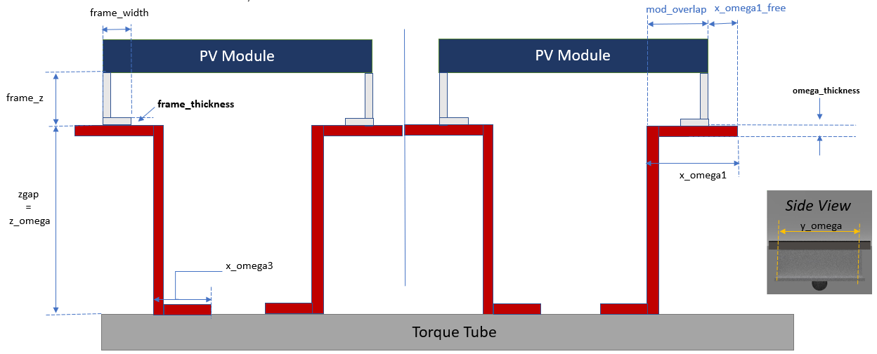
I. Simulating Frames and Omegas#
The values for generating frames and omegas are described in the makeModule function, which is where they are introduced into the basic module unit. This diagram shows how they are measured.
[2]:
module_type = 'test-module'

frameParams = {'frame_material' : 'Metal_Grey',
               'frame_thickness' : 0.05,
               'nSides_frame' : 4,
               'frame_width' : 0.08}

frameParams = {'frame_material' : 'Metal_Grey',
               'frame_thickness' : 0.05,
               'nSides_frame' : 4,
               'frame_width' : 0.08}

omegaParams = {'omega_material': 'litesoil',
                'x_omega1' : 0.4,
                'mod_overlap' : 0.25,
                'y_omega' : 1.5,
                'x_omega3' : 0.25,
                'omega_thickness' : 0.05,
                'inverted' : False}

tubeParams = { 'visible': True,
              'axisofrotation' : True,
              'diameter' : 0.3
             }


demo = bifacial_radiance.RadianceObj('tutorial_15', testfolder)

mymodule = demo.makeModule(module_type,x=2, y=1, xgap = 0.02, ygap = 0.15, zgap = 0.3,
                numpanels = 2, tubeParams=tubeParams,
                frameParams=frameParams, omegaParams=omegaParams)
path = C:\Users\mprillim\sam_dev\bifacial_radiance\bifacial_radiance\TEMP\Tutorial_15
Making path: images
Making path: objects
Making path: results
Making path: skies
Making path: EPWs
Making path: materials

Module Name: test-module
Module test-module updated in module.json
Alternatively, the paremeters can be passed from an Object Oriented Approach as follows:
[3]:
mymodule.addTorquetube(visible = True, axisofrotation = True, diameter = 0.3)

mymodule.addOmega(omega_material = 'litesoil', x_omega1 = 0.4, mod_overlap = 0.25,
                 y_omega = 1.5, x_omega3 = 0.25, omega_thickness = 0.05, inverted = False)

mymodule.addFrame(frame_material = 'Metal_Grey', frame_thickness = 0.05, nSides_frame = 4, frame_width = 0.08)
Module test-module updated in module.json
Pre-existing .rad file objects\test-module.rad will be overwritten

Module test-module updated in module.json
Pre-existing .rad file objects\test-module.rad will be overwritten

Module test-module updated in module.json
Pre-existing .rad file objects\test-module.rad will be overwritten
Let’s add the rest of the scene and go until OCT, so it can be viewed with rvu:
[4]:
demo.setGround(0.2)
epwfile = demo.getEPW(lat = 37.5, lon = -77.6)
metdata = demo.readWeatherFile(epwfile, coerce_year = 2021)
demo.gendaylit(4020)

sceneDict = {'tilt':0, 'pitch':3, 'clearance_height':3,'azimuth':90, 'nMods': 1, 'nRows': 1}
scene = demo.makeScene(mymodule,sceneDict)
demo.makeOct()
Loading albedo, 1 value(s), 0.200 avg
1 nonzero albedo values.
Getting weather file: USA_VA_Richmond.724010_TMY2.epw
 ... OK!
8760 line in WeatherFile. Assuming this is a standard hourly WeatherFile for the year for purposes of saving Gencumulativesky temporary weather files in EPW folder.
Coercing year to 2021
Saving file EPWs\metdata_temp.csv, # points: 8760
Calculating Sun position for Metdata that is right-labeled  with a delta of -30 mins. i.e. 12 is 11:30 sunpos
Created tutorial_15.oct
[4]:
'tutorial_15.oct'
To view the module from different angles, you can use the following rvu commands in your terminal:
rvu -vp -7 0 3 -vd 1 0 0 Sim1.oct


rvu -vp 0 -5 3 -vd 0 1 0 Sim1.oct
[5]:
## Comment any of the ! line below to run rvu from the Jupyter notebook instead of your terminal.
## Simulation will stop until you close the rvu window(s).

#!rvu -vp -7 0 3 -vd 1 0 0 Sim1.oct
#!rvu -vp 0 -5 3 -vd 0 1 0 Sim1.oct
II. Improvements to irradiance sampling#
The key ideas here are:
moduleAnalysis()returns two structured dictionaries that have the coordinates necessary for analysis to know where to smaple. On the new version, different values can be given for sampling accross the collector slope (y), for both front and backs by using a single value or an array insensorsy.Furthermore, now scanning on the module’s x-direction is supported, by setting the variables
sensorsxas an singel value or an array.
When the sensors differ between the front and the back, instead of saving one .csv with results, two .csv files are saved, one labeled “_Front.csv” and the other “_Back.csv”.
To know more, read the functions documentation.
We’ll take advantage of Simulation 1 testfolder, Radiance Objects and sky, but let’s make a simple module and scene and model it through from there.
[6]:
mymodule = demo.makeModule(name='test-module',x=2, y=1)
sceneDict = {'tilt':0, 'pitch':6, 'clearance_height':3,'azimuth':180, 'nMods': 1, 'nRows': 1}
Module Name: test-module
Module test-module updated in module.json
Pre-existing .rad file objects\test-module.rad will be overwritten
[7]:
scene = demo.makeScene(mymodule,sceneDict)
octfile = demo.makeOct()
analysis = bifacial_radiance.AnalysisObj()  # return an analysis object including the scan dimensions for back irradiance
Created tutorial_15.oct
Same sensors front and back, two sensors accross x#
[8]:
name='2222'
sensorsy_front = 2
sensorsy_back = 2
sensorsx_front = 2
sensorsx_back = 2

sensorsy = [sensorsy_front, sensorsy_back]
sensorsx = [sensorsx_front, sensorsx_back]

frontscan, backscan = analysis.moduleAnalysis(scene, sensorsy = sensorsy, sensorsx=sensorsx)

frontDict, backDict = analysis.analysis(octfile = octfile, name = name, frontscan = frontscan,
                                        backscan = backscan)

print('\n--> RESULTS for Front and Back are saved on the same file since the sensors match for front and back')
print('\n', bifacial_radiance.load.read1Result('results\irr_'+name+'_Row1_Module1.csv'))
Linescan in process: 2222_Front
Linescan in process: 2222_Back
Saved: results\irr_2222.csv

--> RESULTS for Front and Back are saved on the same file since the sensors match for front and back

           x         y      z  rearZ                   mattype  \
0 -0.333333 -0.166667  3.021  2.999  a0.0.a0.test-module.6457
1 -0.333333  0.166667  3.021  2.999  a0.0.a0.test-module.6457
2  0.333333 -0.166667  3.021  2.999  a0.0.a0.test-module.6457
3  0.333333  0.166667  3.021  2.999  a0.0.a0.test-module.6457

                    rearMat  Wm2Front   Wm2Back  Back/FrontRatio
0  a0.0.a0.test-module.2310  188.8667  36.90352         0.195393
1  a0.0.a0.test-module.2310  188.8637  36.89747         0.195365
2  a0.0.a0.test-module.2310  188.8633  36.89517         0.195353
3  a0.0.a0.test-module.2310  188.8603  36.88242         0.195288
Different sensors front and back, two sensors accross x#
[11]:
name='2412'

sensorsy_front = 2
sensorsy_back = 4

sensorsx_front = 1
sensorsx_back = 2

sensorsy = [sensorsy_front, sensorsy_back]
sensorsx = [sensorsx_front, sensorsx_back]

frontscan, backscan = analysis.moduleAnalysis(scene, sensorsy=sensorsy, sensorsx=sensorsx)

frontDict, backDict = analysis.analysis(octfile = octfile, name = name, frontscan = frontscan,
                                        backscan = backscan)

print('\n--> RESULTS for Front and Back are saved on SEPARATE file since the sensors do not match for front and back')

print('\nFRONT\n', bifacial_radiance.load.read1Result('results\irr_'+name+'_Row1_Module1_Front.csv'))
print('\nBACK\n', bifacial_radiance.load.read1Result('results\irr_'+name+'_Row1_Module1_Back.csv'))
Linescan in process: 2412_Row1_Module1_Front
Linescan in process: 2412_Row1_Module1_Back
Saved: results\irr_2412_Row1_Module1_Front.csv
Saved: results\irr_2412_Row1_Module1_Back.csv

--> RESULTS for Front and Back are saved on SEPARATE file since the sensors do not match for front and back

FRONT
      x      y      z                   mattype  Wm2Front
0  0.0 -0.167  3.025  a0.0.a0.test-module.6457   187.685
1  0.0  0.167  3.025  a0.0.a0.test-module.6457   187.682

BACK
        x    y      z                   rearMat  Wm2Back
0 -0.333 -0.3  2.994  a0.0.a0.test-module.2310   36.644
1 -0.333 -0.1  2.994  a0.0.a0.test-module.2310   36.632
2 -0.333  0.1  2.994  a0.0.a0.test-module.2310   36.620
3 -0.333  0.3  2.994  a0.0.a0.test-module.2310   36.608
4  0.333 -0.3  2.994  a0.0.a0.test-module.2310   36.640
5  0.333 -0.1  2.994  a0.0.a0.test-module.2310   36.618
6  0.333  0.1  2.994  a0.0.a0.test-module.2310   36.605
7  0.333  0.3  2.994  a0.0.a0.test-module.2310   36.591
III. Making Analysis Function for Row#
Let’s explore how to analyze easily a row with the new function analyzeRow. As before, we are not repeating functions alreayd called above, just re-running the necessary ones to show the changes.
[12]:
sceneDict = {'tilt':0, 'pitch':30, 'clearance_height':3,'azimuth':90, 'nMods': 3, 'nRows': 3}
scene = demo.makeScene(mymodule,sceneDict)
octfile = demo.makeOct()
Append=False in makeScene. Existing scenes being over-written.
Created tutorial_15.oct
The function requires to know the number of modules on the row
[13]:
sensorsy_back=1
sensorsx_back=1
sensorsy_front=1
sensorsx_front=1

sensorsy = [sensorsy_front, sensorsy_back]
sensorsx = [sensorsx_front, sensorsx_back]

rowscan = analysis.analyzeRow(name = name, scene = scene, sensorsy=sensorsy, sensorsx = sensorsx,
                              rowWanted = 1, octfile = octfile)
Linescan in process: 2412_Row1_Module1_Front
Linescan in process: 2412_Row1_Module1_Back
Saved: results\irr_2412_Row1_Module1.csv
Linescan in process: 2412_Row1_Module2_Front
Linescan in process: 2412_Row1_Module2_Back
Saved: results\irr_2412_Row1_Module2.csv
Linescan in process: 2412_Row1_Module3_Front
Linescan in process: 2412_Row1_Module3_Back
Saved: results\irr_2412_Row1_Module3.csv
Making path for compiled results: results\CompiledResults
rowscan is now a dataframe containing the values of each module in the row. Check the x, y and