
[1]:
# This information helps with debugging and getting support :)
import sys, platform
import pandas as pd
import bifacial_radiance as br
print("Working on a ", platform.system(), platform.release())
print("Python version ", sys.version)
print("Pandas version ", pd.__version__)
print("bifacial_radiance version ", br.__version__)
Working on a  Windows 10
Python version  3.11.8 | packaged by conda-forge | (main, Feb 16 2024, 20:40:50) [MSC v.1937 64 bit (AMD64)]
Pandas version  2.2.3
bifacial_radiance version  0.5.0b2.dev4+gedb973d.d20250924
4 - Debugging with Custom Objects#
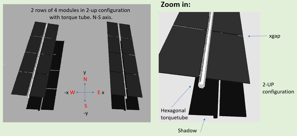
Fixed Tilt 2-up with Torque Tube + CLEAN Routine + CustomObject#
This journal has examples of various things, some which hav ebeen covered before and some in more depth:
Running a fixed_tilt simulation beginning to end.
Creating a 2-up module with torque-tube, and detailed geometry of spacings in xgap, ygap and zgap.
Calculating the tracker angle for a specific time, in case you want to use that value to model a fixed_tilt setup.
Loading and cleaning results, particularly important when using setups with torquetubes / ygaps.
Adding a “Custom Object” or marker at the Origin of the Scene, to do a visual sanity-check of the geometry.
It will look something like this (without the marker in this visualization):
STEPS:
Specify Working Folder and Import Program
Specify all variables
Create the Radiance Object and generate the Sky
Calculating tracker angle/geometry for a specific timestamp
Making the Module & the Scene, Visualize and run Analysis
Calculate Bifacial Ratio (clean results)
Add Custom Elements to your Scene Example: Marker at 0,0 position
1. Specify Working Folder and Import Program#
[2]:
import os
from pathlib import Path

testfolder = Path().resolve().parent.parent / 'bifacial_radiance' / 'TEMP' / 'Tutorial_04'

# Another option using relative address; for some operative systems you might need '/' instead of '\'
# testfolder = os.path.abspath(r'..\..\bifacial_radiance\TEMP')

print ("Your simulation will be stored in %s" % testfolder)

if not os.path.exists(testfolder):
    os.makedirs(testfolder)

import bifacial_radiance
import numpy as np
import pandas as pd
Your simulation will be stored in C:\Users\cdeline\Documents\Python Scripts\Bifacial_Radiance\bifacial_radiance\TEMP\Tutorial_04
2. Specify all variables for the module and scene#
Below find a list of all of the possible parameters for makeModule. scene and simulation parameters are also organized below. This simulation will be a complete simulation in terms of parameters that you can modify.
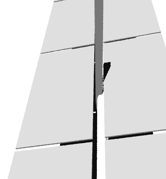
The below routine creates a HEXAGONAL torque tube, for a 2-UP configuration of a specific module size. Parameters for the module, the torque tube, and the scene are below. This is being run with gendaylit, for one specific timestamp
[3]:
simulationname = 'tutorial_4'

## SceneDict Parameters
gcr = 0.33   # ground cover ratio,  = module_height / pitch
albedo = 0.28  #'concrete'     # ground albedo
hub_height = 2.35  # we could also pass clearance_height.
azimuth_ang = 90 # Modules will be facing East.
lat = 37.5
lon = -77.6
nMods = 4   # doing a smaller array for better visualization on this example.
nRows = 2

# MakeModule Parameters
module_type='test-module'
x = 1.996      # landscape, sinze x > y. Remember that orientation has been deprecated.
y = 0.991
tilt = 10
numpanels = 2  # doing a 2-up system!


# Gaps:
xgap = 0.05  # distance between modules in the row.
ygap = 0.15  # distance between the 2 modules along the collector slope.
zgap = 0.175 # if there is a torquetube, this is the distance between the torquetube and the modules.
# If there is not a module, zgap is the distance between the module and the axis of rotation (relevant for
# tracking systems.

# TorqueTube Parameters
tubetype = 'Hex'
diameter = 0.15
material = 'Metal_Grey'       # IT's NOT GRAY, IT's GREY.
3. Create the Radiance Object and generate the Sky#
[4]:
demo = bifacial_radiance.RadianceObj(simulationname, path=str(testfolder))  # Create a RadianceObj 'object'
demo.setGround(albedo) # input albedo number or material name like 'concrete'.  To see options, run this without any input.
epwfile = demo.getEPW(lat,lon) # pull TMY data for any global lat/lon
metdata = demo.readWeatherFile(epwfile, coerce_year=2001) # read in the EPW weather data from above

timestamp = metdata.datetime.index(pd.to_datetime('2001-06-17 13:0:0 -5')) # Make this timezone aware, use -5 for EST.
demo.gendaylit(timestamp)  # Mid-day, June 17th
path = C:\Users\cdeline\Documents\Python Scripts\Bifacial_Radiance\bifacial_radiance\TEMP\Tutorial_04
Making path: images
Making path: objects
Making path: results
Making path: skies
Making path: EPWs
Making path: materials
Loading albedo, 1 value(s), 0.280 avg
1 nonzero albedo values.
Getting weather file: USA_VA_Richmond.724010_TMY2.epw
 ... OK!
8760 line in WeatherFile. Assuming this is a standard hourly WeatherFile for the year for purposes of saving Gencumulativesky temporary weather files in EPW folder.
Coercing year to 2001
Saving file EPWs\metdata_temp.csv, # points: 8760
Calculating Sun position for Metdata that is right-labeled  with a delta of -30 mins. i.e. 12 is 11:30 sunpos
[4]:
'skies\\sky2_37.5_-77.33_2001-06-17_1300.rad'
4. Calculating tracker angle/geometry for a specific timestamp#
This trick is useful if you are trying to use the fixed-tilt steps in bifacial_radiance to model a tracker for one specific point in time (if you take a picture of a tracker, it looks fixed, right? Well then).
We assigned a 10 degree tilt at the beginning, but if we were to model a tracker as a fixed-tilt element because we are interested in only one point in time, this routine will tell us what tilt to use. Please note that to model a tracker as fixed tilt, we suggest passing a hub_height, otherwise you will have to calculate the clearance_height manually.
Details: you might have noticed in the previoust tutorial looking at the tracker dictionary, but the way that bifacial_radiance handles tracking: If the tracker is N-S axis azimuth, the surface azimuth of the modules will be set to 90 always, with a tilt that is either positive (for the early morning, facing East), or negative (for the afternoon, facing west).
[5]:
# Some tracking parameters that won't be needed after getting this angle:
axis_azimuth = 180
axis_tilt = 0
limit_angle = 60
backtrack = True
tilt = demo.getSingleTimestampTrackerAngle(timeindex=timestamp, gcr=gcr, azimuth=axis_azimuth, axis_tilt=axis_tilt, limit_angle=limit_angle, backtrack=backtrack)

print ("\n NEW Calculated Tilt: %s " % tilt)
NEW Calculated Tilt: -4.67
5. Making the Module & the Scene, Visualize and run Analysis#
[6]:
# Making module with all the variables
module = demo.makeModule(name=module_type,x=x,y=y,bifi=1,
                         zgap=zgap, ygap=ygap,  xgap=xgap, numpanels=numpanels)
module.addTorquetube(diameter=diameter, material=material, tubetype=tubetype,
                    visible=True, axisofrotation=True)

# create a scene with all the variables.
# Specifying the pitch automatically with the collector width (sceney) returned by the module object.
# Height has been deprecated as an input. pass clearance_height or hub_height in the scenedict.

sceneDict = {'tilt':tilt,'pitch': np.round(module.sceney / gcr,3),
             'hub_height':hub_height,'azimuth':azimuth_ang,
             'module_type':module_type, 'nMods': nMods, 'nRows': nRows}

scene = demo.makeScene(module=module, sceneDict=sceneDict) #makeScene creates a .rad file of the Scene

octfile = demo.makeOct(demo.getfilelist())  # makeOct combines all of the ground, sky and object files into a .oct file.
Module Name: test-module
Module test-module updated in module.json
Module test-module updated in module.json
Pre-existing .rad file objects\test-module.rad will be overwritten

Created tutorial_4.oct
At this point you should be able to go into a command window (cmd.exe) and check the geometry. It should look like the image at the beginning of the journal. Example:
rvu -vf views:nbsphinx-math:`front`.vp -e .01 -pe 0.02 -vp -2 -12 14.5 tutorial_4.oct*
[7]:
## Comment the line below to run rvu from the Jupyter notebook instead of your terminal.
## Simulation will stop until you close the rvu window

#!rvu -vf views\front.vp -e .01 tutorial_4.oct
And then proceed happily with your analysis:
[8]:
analysis = bifacial_radiance.AnalysisObj(octfile, demo.name)  # return an analysis object including the scan dimensions for back irradiance

sensorsy = 200 # setting this very high to see a detailed profile of the irradiance, including
#the shadow of the torque tube on the rear side of the module.
frontscan, backscan = analysis.moduleAnalysis(scene, modWanted = 2, rowWanted = 1, sensorsy = 200)
frontDict, backDict = analysis.analysis(octfile, demo.name, frontscan, backscan)  # compare the back vs front irradiance

# print('"Annual" bifacial ratio average:  %0.3f' %( sum(analysis.Wm2Back) / sum(analysis.Wm2Front) ) )
# See comment below of why this line is commented out.
Linescan in process: tutorial_4_Row1_Module2_Front
Linescan in process: tutorial_4_Row1_Module2_Back
Saved: results\irr_tutorial_4_Row1_Module2.csv
6. Calculate Bifacial Ratio (clean results)#
Although we could calculate a bifacial ratio average at this point, this value would be misleading, since some of the sensors generated will fall on the torque tube, the sky, and/or the ground since we have torquetube and ygap in the scene. To calculate the real bifacial ratio average, we must use the clean routines.
[11]:
resultFile='results/irr_tutorial_4_Row1_Module2.csv'
results_loaded = bifacial_radiance.load.read1Result(resultFile)
print("Printing the dataframe containing the results just calculated in %s: " % resultFile)
results_loaded
Printing the dataframe containing the results just calculated in results/irr_tutorial_4_Row1_Module2.csv:
[11]:
| x | y | z | rearZ | mattype | rearMat | Wm2Front | Wm2Back | Back/FrontRatio | rearX | rearY | |
|---|---|---|---|---|---|---|---|---|---|---|---|
| 0 | 1.029 | 0.0 | 2.710 | 2.680 | a1.0.a0.test-module.6457 | a1.0.a0.test-module.2310 | 909.867 | 186.261 | 0.205 | 1.032 | 0.0 |
| 1 | 1.019 | 0.0 | 2.710 | 2.680 | a1.0.a0.test-module.6457 | a1.0.a0.test-module.2310 | 909.868 | 186.047 | 0.204 | 1.021 | 0.0 |
| 2 | 1.008 | 0.0 | 2.709 | 2.678 | a1.0.a0.test-module.6457 | a1.0.a0.test-module.2310 | 909.868 | 185.849 | 0.204 | 1.011 | 0.0 |
| 3 | 0.998 | 0.0 | 2.709 | 2.678 | a1.0.a0.test-module.6457 | a1.0.a0.test-module.2310 | 909.868 | 185.635 | 0.204 | 1.000 | 0.0 |
| 4 | 0.987 | 0.0 | 2.707 | 2.676 | a1.0.a0.test-module.6457 | a1.0.a0.test-module.2310 | 909.868 | 185.431 | 0.204 | 0.990 | 0.0 |
| ... | ... | ... | ... | ... | ... | ... | ... | ... | ... | ... | ... |
| 195 | -1.033 | 0.0 | 2.543 | 2.512 | a1.0.a1.test-module.6457 | a1.0.a1.test-module.2310 | 909.878 | 185.560 | 0.204 | -1.030 | 0.0 |
| 196 | -1.043 | 0.0 | 2.541 | 2.510 | a1.0.a1.test-module.6457 | a1.0.a1.test-module.2310 | 909.878 | 185.743 | 0.204 | -1.040 | 0.0 |
| 197 | -1.055 | 0.0 | 2.541 | 2.510 | a1.0.a1.test-module.6457 | a1.0.a1.test-module.2310 | 909.878 | 185.958 | 0.204 | -1.052 | 0.0 |
| 198 | -1.064 | 0.0 | 2.540 | 2.508 | a1.0.a1.test-module.6457 | a1.0.a1.test-module.2310 | 909.878 | 186.141 | 0.205 | -1.062 | 0.0 |
| 199 | -1.074 | 0.0 | 2.540 | 2.508 | a1.0.a1.test-module.6457 | a1.0.a1.test-module.2310 | 909.878 | 186.144 | 0.205 | -1.071 | 0.0 |
200 rows × 11 columns
[12]:
print("Looking at only 1 sensor in the middle -- position 100 out of the 200 sensors sampled:")
results_loaded.loc[100]
Looking at only 1 sensor in the middle -- position 100 out of the 200 sensors sampled:
[12]:
x                               -0.028
y                                  0.0
z                                2.625
rearZ                            2.594
mattype            a1.0.hextube1a.6457
rearMat                            sky
Wm2Front                       814.726
Wm2Back                        161.885
Back/FrontRatio                  0.199
rearX                           -0.025
rearY                              0.0
Name: 100, dtype: object
As an example, we can see above that sensor 100 falls in the hextube, and in the sky. We need to remove this to calculate the real bifacial_gain from the irradiance falling into the modules. To do this we use cleanResult form the load.py module in bifacial_radiance. This finds the invalid materials and sets the irradiance values for those materials to NaN
This might take some time in the current version.
[13]:
# Cleaning Results:
# remove invalid materials and sets the irradiance values to NaN
clean_results = bifacial_radiance.load.cleanResult(results_loaded)
[14]:
print("Sampling the same location as before to see what the results are now:")
clean_results.loc[100]
Sampling the same location as before to see what the results are now:
[14]:
x                               -0.028
y                                  0.0
z                                2.625
rearZ                            2.594
mattype            a1.0.hextube1a.6457
rearMat                            sky
Wm2Front                           NaN
Wm2Back                            NaN
Back/FrontRatio                  0.199
rearX                           -0.025
rearY                              0.0
Name: 100, dtype: object
[15]:
print('CORRECT Annual bifacial ratio average:  %0.3f' %( clean_results['Wm2Back'].sum() / clean_results['Wm2Front'].sum() ))

print ("\n(If we had not done the cleaning routine, the bifacial ratio would have been ", \
      "calculated to %0.3f  <-- THIS VALUE IS WRONG)" %( sum(analysis.Wm2Back) / sum(analysis.Wm2Front) ))
CORRECT Annual bifacial ratio average:  0.200

(If we had not done the cleaning routine, the bifacial ratio would have been  calculated to 0.202  <-- THIS VALUE IS WRONG)
7. Add Custom Elements to your Scene Example: Marker at 0,0 position#
This shows how to add a custom element, in this case a Cube, that will be placed in the center of your already created scene to mark the 0,0 location.
This can be added at any point after makeScene has been run once. Notice that if this extra element is in the scene and the analysis sensors fall on this element, they will measure irradiance at this element and no the modules. New in v0.5.0: Multiple sceneobjects can be added to the scene, using customtext parameter and append=True.
We are going to create a “MyMarker.rad” file in the objects folder, right after we make the Module. This is a prism (so we use ‘genbox’), that is black from the ground.rad list of materials (‘black’) We are naming it ‘CenterMarker’ Its sides are going to be 0.5x0.5x0.5 m and We are going to leave its bottom surface coincident with the plane z=0, but going to center on X and Y.
[16]:
name='MyMarker'
text='! genbox black CenterMarker 0.1 0.1 4 | xform -t -0.05 -0.05 0'
customObject = demo.makeCustomObject(name,text)
Custom Object Name objects\MyMarker.rad
This should have created a MyMarker.rad object on your objects folder.
But creating the object does not automatically adds it to the scene. So let’s now add the customObject to the Scene. We are not going to translate it or anything because we want it at the center, but you can pass translation, rotation, and any other XFORM command from Radiance. The custom object is added to the scene .rad file.
Starting in v0.5.0 we can have multiple scenes, and these are now stored in the array demo.scenes.
[19]:
demo.scenes[0]
[19]:
<class 'bifacial_radiance.main.SceneObj'> : {'gcr': np.float64(0.32998), 'hpc': False, 'module': <class 'bifacial_radiance.module.ModuleObj'> : {'x': 1.996, 'y': 0.991, 'z': 0.02, 'modulematerial': 'black', 'scenex': np.float64(2.046), 'sceney': np.float64(2.132), 'scenez': np.float64(0.25), 'numpanels': 2, 'bifi': 1, 'text': '! genbox black test-module 1.996 0.991 0.02 | xform -t -0.998 -1.066 0.25 -a 2 -t 0 1.141 0\r\n! genbox Metal_Grey hextube1a 2.046 0.075 0.129904 | xform -t -1.023 -0.0375 -0.064952\r\n! genbox Metal_Grey hextube1b 2.046 0.075 0.129904 | xform -t -1.023 -0.0375 0.064952 -rx 60 -t 0 0 0\r\n! genbox Metal_Grey hextube1c 2.046 0.075 0.129904 | xform -t -1.023 -0.0375 -0.064952 -rx -60 -t 0 0 0', 'modulefile': 'objects\\test-module.rad', 'glass': False, 'glassEdge': 0.01, 'offsetfromaxis': np.float64(0.25), 'xgap': 0.05, 'ygap': 0.15, 'zgap': 0.175}, 'modulefile': 'objects\\test-module.rad', 'name': 'Scene0', 'radfiles': ['objects\\test-module_C_2.28_rtr_6.46_tilt_-5_4modsx2rows_origin0,0.rad'], 'sceneDict': {'tilt': -4.67, 'pitch': np.float64(6.461), 'hub_height': 2.35, 'azimuth': 90, 'module_type': 'test-module', 'nMods': 4, 'nRows': 2, 'axis_tilt': 0, 'originx': 0, 'originy': 0}, 'text': '!xform -rx -4.67 -t 0 0 2.35 -a 4 -t 2.046 0 0 -a 2 -t 0 6.461 0 -i 1 -t -2.046 -0.0 0 -rz 90 -t 0 0 0 "objects\\test-module.rad"'}
[27]:
demo.scenes[0].radfiles
[27]:
['objects\\test-module_C_2.28_rtr_6.46_tilt_-5_4modsx2rows_origin0,0.rad']
[30]:
# Append the custom object.  It should now show up in the scene radfile.
scene = demo.scenes[0].appendtoScene(customObject=customObject)
[29]:
# makeOct combines all of the ground, sky and object files into a .oct file.
octfile = demo.makeOct(demo.getfilelist())
Created tutorial_4.oct
appendtoScene appended to the Scene.rad file the name of the custom object we created and the xform transformation we included as text. Then octfile merged this new scene with the ground and sky files.
At this point you should be able to go into a command window (cmd.exe) and check the geometry, and the marker should be there.
[ ]:
## Comment the line below to run rvu from the Jupyter notebook instead of your terminal.
## Simulation will stop until you close the rvu window

#!rvu -vf views\front.vp -e .01 tutorial_4.oct
If you ran the getTrackerAngle detour and appended the marker, it should look like this:
If you do an analysis and any of the sensors hits the Box object we just created, the list of materials in the result.csv file should say something with “CenterMarker” on it.
See more examples of the use of makeCustomObject and appendtoScene on the Bifacial Carport/Canopies Tutorial