[ ]:

# This information helps with debugging and getting support :)
import sys, platform
import pandas as pd
import bifacial_radiance as br
print("Working on a ", platform.system(), platform.release())
print("Python version ", sys.version)
print("Pandas version ", pd.__version__)
print("bifacial_radiance version ", br.__version__)

13 - Modeling Modules with Glass#

This journal shows how to add glass to the modules. It also shows how to sample irradiance on the surface of the glass, as well as on the surface of the module. Surface of the module is slightlyt less irradiance due to fresnel losses (a.k.a. Angle of Incidence losses (AOI))

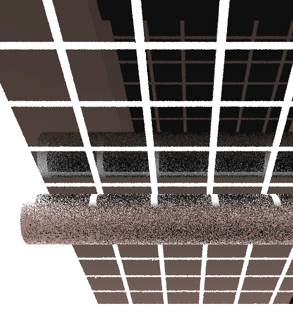
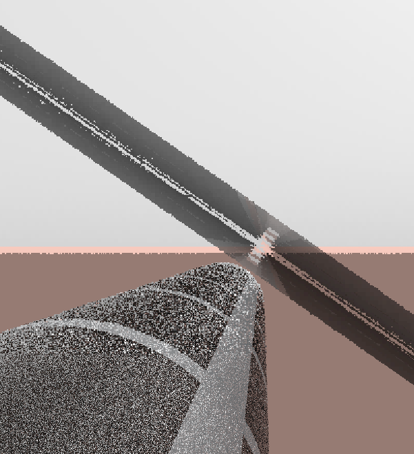
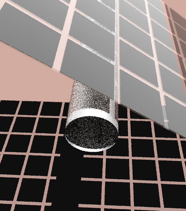
Some examples of the module with glass we’ll create:

Bottom Reflection Side closeup Tiled view

[1]:

import os
from bifacial_radiance import *
from pathlib import Path

testfolder = str(Path().resolve().parent.parent / 'bifacial_radiance' / 'TEMP' / 'Tutorial_13')
if not os.path.exists(testfolder):
    os.makedirs(testfolder)

print ("Your simulation will be stored in %s" % testfolder)

Your simulation will be stored in C:\Users\mprillim\sam_dev\bifacial_radiance\bifacial_radiance\TEMP\Tutorial_13

[2]:

demo = RadianceObj('tutorial_13',str(testfolder))
demo.setGround(0.30)  # This prints available materials.
epwfile = demo.getEPW(lat = 37.5, lon = -77.6)  # This location corresponds to Richmond, VA.
metdata = demo.readWeatherFile(epwfile)
demo.gendaylit(8)  # January 1 4pm (timepoint # 8)\

path = C:\Users\mprillim\sam_dev\bifacial_radiance\bifacial_radiance\TEMP\Tutorial_13
Loading albedo, 1 value(s), 0.300 avg
1 nonzero albedo values.
Getting weather file: USA_VA_Richmond.724010_TMY2.epw
 ... OK!
8760 line in WeatherFile. Assuming this is a standard hourly WeatherFile for the year for purposes of saving Gencumulativesky temporary weather files in EPW folder.
Coercing year to 2021
Saving file EPWs\metdata_temp.csv, # points: 8760
Calculating Sun position for Metdata that is right-labeled  with a delta of -30 mins. i.e. 12 is 11:30 sunpos

[2]:

'skies\\sky2_37.5_-77.33_2021-01-01_1600.rad'

Modeling example with glass#

[3]:

module_type = 'test-module'

numcellsx = 6
numcellsy = 12
xcell = 0.156
ycell = 0.156
xcellgap = 0.02
ycellgap = 0.02

visible = True
diameter = 0.15
tubetype = 'round'
material = 'Metal_Grey'
xgap = 0.1
ygap = 0
zgap = 0.05
numpanels = 1
axisofrotationTorqueTube = False
glass = True

cellLevelModuleParams = {'numcellsx': numcellsx, 'numcellsy':numcellsy,
                         'xcell': xcell, 'ycell': ycell, 'xcellgap': xcellgap, 'ycellgap': ycellgap}

mymodule = demo.makeModule(name=module_type, x=1, y=1, xgap=xgap, ygap=ygap,
                           zgap=zgap, numpanels=numpanels, glass=glass, z=0.0002)
mymodule.addTorquetube(material=material, tubetype=tubetype, diameter=diameter,
                      axisofrotation=axisofrotationTorqueTube, recompile=False)
mymodule.addCellModule(**cellLevelModuleParams)

sceneDict = {'tilt':0,'pitch':5.5,'hub_height':1.0,'azimuth':90, 'nMods': 20, 'nRows': 1, 'originx':0, 'originy':0}
scene = demo.makeScene(module_type, sceneDict)
octfile = demo.makeOct(demo.getfilelist())


Module Name: test-module

Warning: module glass increases analysis variability. Recommend setting `accuracy='high'` in AnalysisObj.analysis().

Module test-module updated in module.json
Pre-existing .rad file objects\test-module.rad will be overwritten


Warning: module glass increases analysis variability. Recommend setting `accuracy='high'` in AnalysisObj.analysis().

Module was shifted by 0.078 in X to avoid sensors on air
This is a Cell-Level detailed module with Packaging Factor of 0.81 %
Module test-module updated in module.json
Pre-existing .rad file objects\test-module.rad will be overwritten

Created tutorial_13.oct

Advanced Rendering:#

The images at the beginning of the journal can be made pretty with advanced rendering. This is the workflow:

rvu -> rpict -> pcond -> pfilt -> ra_tiff -> convert

In detail:

1. Use rvu to view the oct file

rvu 1axis_07_01_08.oct

Use aim and origin to move around, zoom in/out, etc. Save a view file with view render.

2. Run rpict to render the image to hdr

This is the time consuming step. It takes between 1 and 3 hours depending on how complex the geometry is.

rpict -x 4800 -y 4800 -i -ps 1 -dp 530 -ar 964 -ds 0.016 -dj 1 -dt 0.03 -dc 0.9 -dr 5 -st 0.12 -ab 5 -aa 0.11 -ad 5800 -as 5800 -av 25 25 25 -lr 14 -lw 0.0002 -vf render.vf bifacial_example.oct > render.hdr

3. Run pcond to mimic human visual response

pcond -h render.hdr > render.pcond.hdr

4. Resize and adjust exposure with pfilt

pfilt -e +0.2 -x /4 -y /4 render.pcond.hdr > render.pcond.pfilt.hdr

5. Convert hdr to tif

ra_tiff render.pcond.pfilt.hdr render.tif

6. Convert tif to png with imagemagick convert utility

convert render.tif render.png

7. Annotate the image with convert

convert render.png -fill black -gravity South -annotate +0+5 'Created with NREL bifacial_radiance https://github.com/NatLabRockies/bifacial_radiance' render_annotated.png

[4]:

analysis = AnalysisObj(octfile, demo.basename)

Scanning Outside of the module, the surface of the glass#

[5]:

frontscan, backscan = analysis.moduleAnalysis(scene)
results = analysis.analysis(octfile, demo.basename, frontscan, backscan)
load.read1Result('results\irr_tutorial_13_Row1_Module10.csv')

Linescan in process: tutorial_13_Row1_Module10_Front
Linescan in process: tutorial_13_Row1_Module10_Back
Saved: results\irr_tutorial_13_Row1_Module10.csv

[5]:

	x	z	rearZ	mattype	rearMat	Wm2Front	Wm2Back	Back/FrontRatio	rearX
0	0.837	1.006	0.995	a9.0.a2.1.0.cellPVmodule.6457	a9.0.a0.test-module_Glass.2310	86.163	12.782	0.148	0.837
1	0.628	1.006	0.995	a9.0.a2.2.0.cellPVmodule.6457	a9.0.a0.test-module_Glass.2310	86.164	12.161	0.141	0.628
2	0.418	1.006	0.995	a9.0.a2.3.0.cellPVmodule.6457	a9.0.a0.test-module_Glass.2310	86.165	11.420	0.133	0.418
3	0.209	1.006	0.995	a9.0.a2.4.0.cellPVmodule.6457	a9.0.a0.test-module_Glass.2310	86.166	10.508	0.122	0.209
4	0.000	1.006	0.995	a9.0.a0.test-module_Glass.6457	a9.0.a0.test-module_Glass.2310	85.927	28.141	0.327	0.000
5	-0.209	1.006	0.995	a9.0.a2.7.0.cellPVmodule.6457	a9.0.a0.test-module_Glass.2310	86.168	10.991	0.128	-0.209
6	-0.419	1.006	0.995	a9.0.a2.8.0.cellPVmodule.6457	a9.0.a0.test-module_Glass.2310	86.169	11.858	0.138	-0.419
7	-0.628	1.006	0.995	a9.0.a2.9.0.cellPVmodule.6457	a9.0.a0.test-module_Glass.2310	86.170	12.704	0.147	-0.628
8	-0.837	1.006	0.995	a9.0.a2.10.0.cellPVmodule.6457	a9.0.a0.test-module_Glass.2310	86.171	13.369	0.155	-0.837

Scanning Inside of the module, the surface of the cells#

[8]:

frontscan, backscan = analysis.moduleAnalysis(scene, frontsurfaceoffset=0.05, backsurfaceoffset = 0.05)
results = analysis.analysis(octfile, demo.basename, frontscan, backscan)
load.read1Result('results\irr_tutorial_13_Row1_Module10.csv')

Linescan in process: tutorial_13_Row1_Module10_Front
Linescan in process: tutorial_13_Row1_Module10_Back
Saved: results\irr_tutorial_13_Row1_Module10.csv

[8]:

	x	z	rearZ	mattype	rearMat	Wm2Front	Wm2Back	Back/FrontRatio	rearX
0	0.837	1.051	0.95	a9.0.a2.1.0.cellPVmodule.6457	a9.0.a0.test-module_Glass.2310	86.157	12.887	0.150	0.837
1	0.628	1.051	0.95	a9.0.a2.2.0.cellPVmodule.6457	a9.0.a0.test-module_Glass.2310	86.158	12.266	0.142	0.628
2	0.418	1.051	0.95	a9.0.a2.3.0.cellPVmodule.6457	a9.0.a0.test-module_Glass.2310	86.159	11.481	0.133	0.418
3	0.209	1.051	0.95	a9.0.a2.4.0.cellPVmodule.6457	a9.0.a0.test-module_Glass.2310	86.160	10.462	0.121	0.209
4	0.000	1.051	0.95	a9.0.a0.test-module_Glass.6457	a9.0.a0.test-module_Glass.2310	85.921	28.141	0.328	0.000
5	-0.209	1.051	0.95	a9.0.a2.7.0.cellPVmodule.6457	a9.0.a0.test-module_Glass.2310	86.162	10.956	0.127	-0.209
6	-0.419	1.051	0.95	a9.0.a2.8.0.cellPVmodule.6457	a9.0.a0.test-module_Glass.2310	86.163	11.831	0.137	-0.419
7	-0.628	1.051	0.95	a9.0.a2.9.0.cellPVmodule.6457	a9.0.a0.test-module_Glass.2310	86.164	12.698	0.147	-0.628
8	-0.837	1.051	0.95	a9.0.a2.10.0.cellPVmodule.6457	a9.0.a0.test-module_Glass.2310	86.165	13.377	0.155	-0.837

[ ]: