
[ ]:
# This information helps with debugging and getting support :)
import sys, platform
import pandas as pd
import bifacial_radiance as br
print("Working on a ", platform.system(), platform.release())
print("Python version ", sys.version)
print("Pandas version ", pd.__version__)
print("bifacial_radiance version ", br.__version__)
11 - AgriPV Systems#
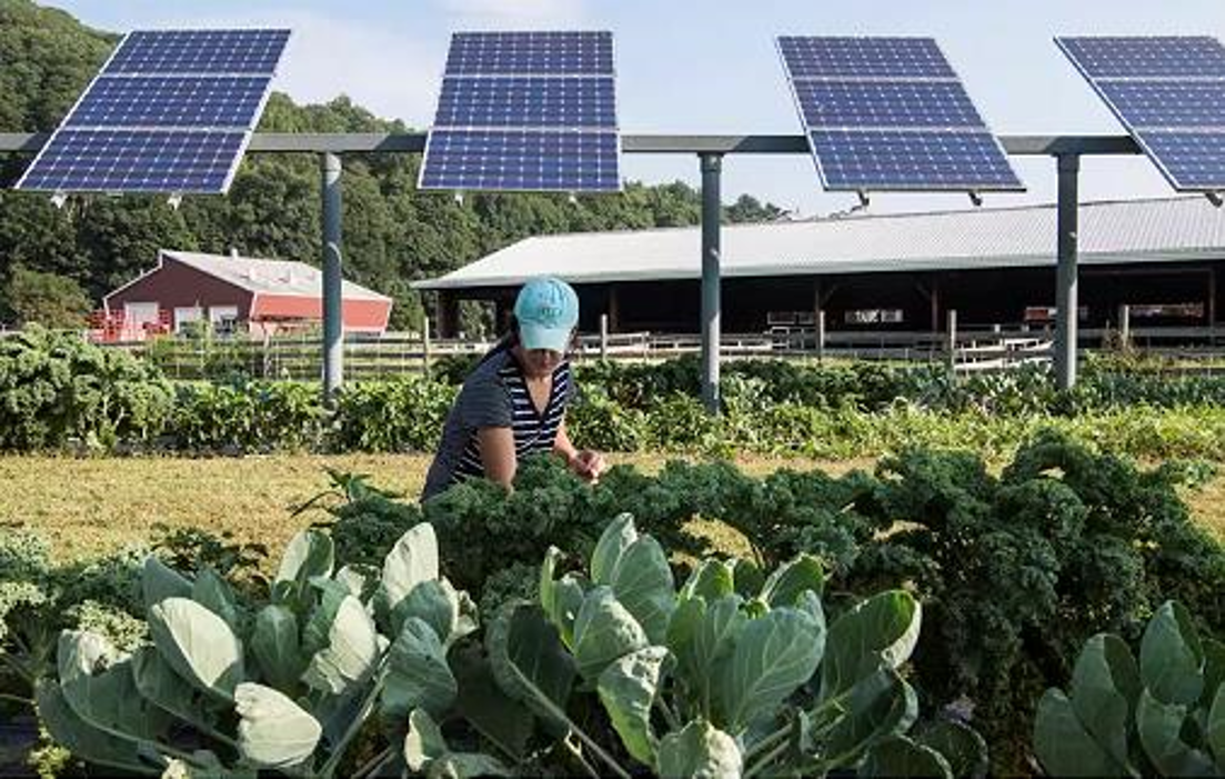
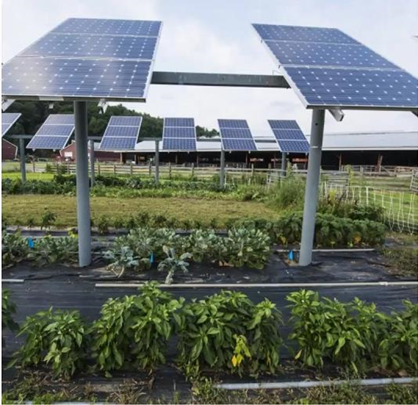
This journal shows how to model an AgriPV site, calculating the irradiance not only on the modules but also the irradiance received by the ground to evaluate available solar ersource for plants.
We assume that bifacia_radiacne is already installed in your computer. This works for bifacial_radiance v.3 release.
These journal outlines 4 useful uses of bifacial_radiance and some tricks:
Creating the modules in the AgriPV site
Adding extra geometry for the pillars/posts supporting the AgriPV site
Hacking the sensors to sample the ground irradiance and create irradiance map
Adding object to simulate variations in ground albedo from different crops between rows.
Steps:#
Generate the geometry
Analyse the Ground Irradiance
Analyse and MAP the Ground Irradiance
Adding different Albedo Section
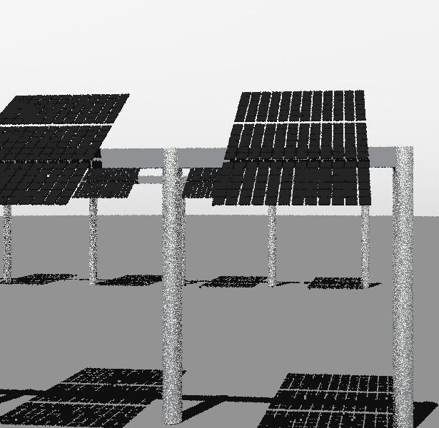
Preview of what we will create:#
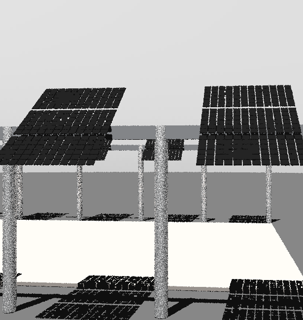
 And this is how it will look like:
1. Generate the geometry#
This section goes from setting up variables to making the OCT axis. We are also adding some custom elements for the torquetubes and posts.
We’ve done this before a couple times, no new stuff here.
The magic is that, for doing the carport we see in the figure, we are going to do a 4-up configuration of modules (numpanels), and we are going to repeat that 3-UP 6 times (nMods)
[1]:
import os
from pathlib import Path

testfolder = str(Path().resolve().parent.parent / 'bifacial_radiance' / 'TEMP' /  'Tutorial_11')

if not os.path.exists(testfolder):
    os.makedirs(testfolder)

print ("Your simulation will be stored in %s" % testfolder)
Your simulation will be stored in C:\Users\cdeline\Documents\Python Scripts\Bifacial_Radiance\bifacial_radiance\TEMP\Tutorial_11
[2]:
import bifacial_radiance as br
import numpy as np
import pandas as pd
import seaborn as sns
from matplotlib import pyplot as plt
[3]:
simulationname = 'tutorial_11'
#Location:
lat = 40.0583 # NJ
lon = -74.4057 # NJ
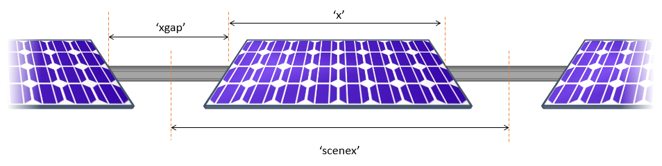
# MakeModule Parameters
moduletype='test-module'
numpanels = 3 # AgriPV site has 3 modules along the y direction (N-S since we are facing it to the south) .
x = 0.95
y = 1.95
xgap = 2.0# Leaving 15 centimeters between modules on x direction
ygap = 0.10 # Leaving 10 centimeters between modules on y direction
zgap = 0 # no gap to torquetube.
sensorsy = 6*numpanels # this will give 6 sensors per module, 1 per cell
# Other default values:
# TorqueTube Parameters
axisofrotationTorqueTube=False # this is False by default if there is no torquetbue parameters
torqueTube = False
cellLevelModule = True
numcellsx = 12
numcellsy = 6
xcell = 0.156
ycell = 0.156
xcellgap = 0.02
ycellgap = 0.02
cellLevelModuleParams = {'numcellsx': numcellsx, 'numcellsy':numcellsy,
'xcell': xcell, 'ycell': ycell, 'xcellgap': xcellgap, 'ycellgap': ycellgap}
# SceneDict Parameters
pitch = 15 # m
albedo = 0.2 #'grass' # ground albedo
hub_height = 4.3 # m
nMods = 6 # six modules per row.
nRows = 3 # 3 row
azimuth_ang=180 # Facing south
tilt =35 # tilt.
# Now let's run the example
demo = br.RadianceObj(simulationname,path = testfolder)
demo.setGround(albedo)
epwfile = demo.getEPW(lat, lon) # NJ lat/lon 40.0583° N, 74.4057
metdata = demo.readWeatherFile(epwfile, coerce_year=2001)
timestamp = metdata.datetime.index(pd.to_datetime('2001-06-17 13:0:0 -5')) # Make this timezone aware, use -5 for EST.
demo.gendaylit(timestamp)
# Making module with all the variables
module=demo.makeModule(name=moduletype,x=x,y=y,numpanels=numpanels,
xgap=xgap, ygap=ygap, cellModule=cellLevelModuleParams)
# create a scene with all the variables
sceneDict = {'tilt':tilt,'pitch': 15,'hub_height':hub_height,'azimuth':azimuth_ang, 'nMods': nMods, 'nRows': nRows}
scene = demo.makeScene(module=moduletype, sceneDict=sceneDict)
octfile = demo.makeOct(demo.getfilelist())
path = C:\Users\cdeline\Documents\Python Scripts\Bifacial_Radiance\bifacial_radiance\TEMP\Tutorial_11
Loading albedo, 1 value(s), 0.200 avg
1 nonzero albedo values.
Getting weather file: USA_NJ_McGuire.AFB.724096_TMY3.epw
 ... OK!
8760 line in WeatherFile. Assuming this is a standard hourly WeatherFile for the year for purposes of saving Gencumulativesky temporary weather files in EPW folder.
Coercing year to 2001
Saving file EPWs\metdata_temp.csv, # points: 8760
Calculating Sun position for Metdata that is right-labeled  with a delta of -30 mins. i.e. 12 is 11:30 sunpos

Module Name: test-module
Module was shifted by 0.078 in X to avoid sensors on air
This is a Cell-Level detailed module with Packaging Factor of 0.81
Module test-module updated in module.json
Pre-existing .rad file objects\test-module.rad will be overwritten

Created tutorial_11.oct
If desired, you can view the Oct file at this point:
rvu -vf views:nbsphinx-math:`front`.vp -e .01 tutorial_11.oct
[4]:
## Comment the ! line below to run rvu from the Jupyter notebook instead of your terminal.
## Simulation will stop until you close the rvu window

#!rvu -vf views\front.vp -e .01 tutorial_11.oct
And adjust the view parameters, you should see this image.
Adding the structure#
We will add on the torquetube and pillars.
Positions of the piles could be done more programatically, but they are kinda estimated at the moment.
[5]:
torquetubelength = module.scenex*(nMods)

name='Post1'
text='! genbox Metal_Aluminum_Anodized torquetube_row1 {} 0.2 0.3 | xform -t {} -0.1 -0.3 | xform -t 0 0 4.2'.format(
                                                    torquetubelength, (-torquetubelength+module.sceney)/2.0)
customObject = demo.makeCustomObject(name,text)
scene.appendtoScene(radfile=scene.radfiles[0],customObject=customObject)

name='Post2'
text='! genbox Metal_Aluminum_Anodized torquetube_row2 {} 0.2 0.3 | xform -t {} -0.1 -0.3 | xform -t 0 15 4.2'.format(
                                            torquetubelength, (-torquetubelength+module.sceney)/2.0)
customObject = demo.makeCustomObject(name,text)
scene.appendtoScene(customObject=customObject)

name='Post3'
text='! genbox Metal_Aluminum_Anodized torquetube_row2 {} 0.2 0.3 | xform -t {} -0.1 -0.3 | xform -t 0 -15 4.2'.format(
                                              torquetubelength, (-torquetubelength+module.sceney)/2.0)
customObject = demo.makeCustomObject(name,text)
scene.appendtoScene(customObject=customObject)
Custom Object Name objects\Post1.rad

Custom Object Name objects\Post2.rad

Custom Object Name objects\Post3.rad
[6]:
name='Pile'
pile1x = (torquetubelength+module.sceney)/2.0
pilesep = pile1x*2.0/7.0

text= '! genrev Metal_Grey tube1row1 t*4.2 0.15 32 | xform -t {} 0 0'.format(pile1x)
text += '\r\n! genrev Metal_Grey tube1row2 t*4.2 0.15 32 | xform -t {} 15 0'.format(pile1x)
text += '\r\n! genrev Metal_Grey tube1row3 t*4.2 0.15 32 | xform -t {} -15 0'.format(pile1x)

for i in range (1, 7):
    text += '\r\n! genrev Metal_Grey tube{}row1 t*4.2 0.15 32 | xform -t {} 0 0'.format(i+1, pile1x-pilesep*i)
    text += '\r\n! genrev Metal_Grey tube{}row2 t*4.2 0.15 32 | xform -t {} 15 0'.format(i+1, pile1x-pilesep*i)
    text += '\r\n! genrev Metal_Grey tube{}row3 t*4.2 0.15 32 | xform -t {} -15 0'.format(i+1, pile1x-pilesep*i)

customObject = demo.makeCustomObject(name,text)
scene.appendtoScene( customObject=customObject)

octfile = demo.makeOct()  # makeOct combines all of the ground, sky and object files we just added into a .oct file.
Custom Object Name objects\Pile.rad
Created tutorial_11.oct
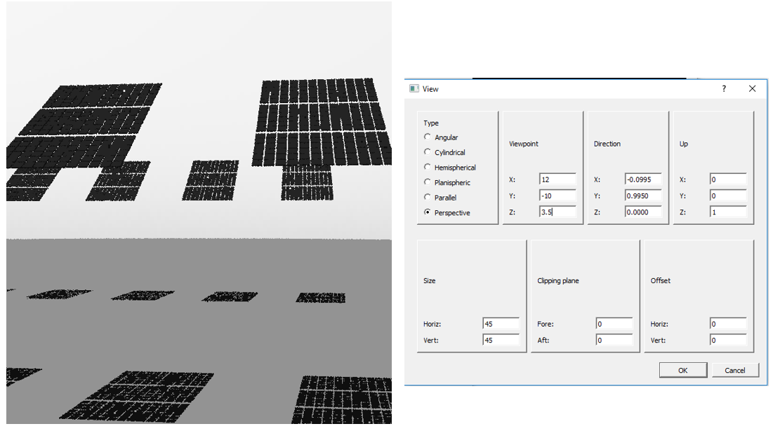
View the geometry with the posts on :#
rvu -vf views:nbsphinx-math:`front`.vp -e .01 -pe 0.4 -vp 12 -10 3.5 -vd -0.0995 0.9950 0.0 tutorial_11.oct
[7]:
## Comment the ! line below to run rvu from the Jupyter notebook instead of your terminal.
## Simulation will stop until you close the rvu window

#!rvu -vf views\front.vp -e .01 tutorial_11.oct
2. Analyse the Ground Irradiance#
Now let’s do some analysis along the ground, starting from the edge of the modules. We wil select to start in the center of the array.
We are also increasign the number of points sampled accross the collector width, with the variable sensorsy passed to moduleanalysis. We are also increasing the step between sampling points, to be able to sample in between the rows.
We’ll use the new ``AnalysisObj.groundAnalysis()`` function starting in v0.5.0 to determine the scan points on the ground.
[8]:
analysis = br.AnalysisObj(octfile, demo.name)
sensorsy = 20
frontscan, backscan = analysis.moduleAnalysis(scene, sensorsy=sensorsy)
groundscan = analysis.groundAnalysis(scene, sensorsground=sensorsy)
groundscan
[8]:
{'xstart': np.float16(0.0),
 'ystart': np.float16(0.0),
 'zstart': np.float16(0.05),
 'xinc': np.float16(0.0),
 'yinc': np.float16(-0.7896),
 'zinc': np.float16(0.0),
 'sx_xinc': 0.0,
 'sx_yinc': 0.0,
 'sx_zinc': 0.0,
 'Nx': 1,
 'Ny': 20,
 'Nz': 1,
 'orient': '0 0 -1'}
[9]:
analysis.analysis(octfile, simulationname+"_scan", groundscan) # compare the back vs front irradiance
Linescan in process: tutorial_11_scan_Row2_Module3_Front
Saved: results\irr_tutorial_11_scan_Row2_Module3.csv
[9]:
{'Wm2': array([332.89396667, 691.32513333, 715.60123333, 735.5388    ,
        744.5296    , 749.1159    , 750.81526667, 752.03366667,
        751.96643333, 747.43736667, 743.95496667, 738.61256667,
        734.60366667, 723.0667    , 708.3394    , 696.8361    ,
        342.9871    , 323.97993333, 317.4839    , 337.0623    ]),
 'x': array([0., 0., 0., 0., 0., 0., 0., 0., 0., 0., 0., 0., 0., 0., 0., 0., 0.,
        0., 0., 0.]),
 'y': array([  0.    ,  -0.7896,  -1.579 ,  -2.37  ,  -3.158 ,  -3.947 ,
         -4.74  ,  -5.527 ,  -6.316 ,  -7.105 ,  -7.895 ,  -8.69  ,
         -9.48  , -10.266 , -11.055 , -11.84  , -12.63  , -13.42  ,
        -14.21  , -15.    ]),
 'z': array([0.05, 0.05, 0.05, 0.05, 0.05, 0.05, 0.05, 0.05, 0.05, 0.05, 0.05,
        0.05, 0.05, 0.05, 0.05, 0.05, 0.05, 0.05, 0.05, 0.05]),
 'r': array([332.7998, 691.1785, 715.4303, 735.3883, 744.4058, 749.002 ,
        750.7009, 751.9545, 751.8872, 747.358 , 743.8846, 738.5325,
        734.5281, 722.988 , 708.2579, 696.7358, 342.8804, 323.8683,
        317.3708, 336.9688]),
 'g': array([332.8915, 691.3184, 715.5896, 735.5281, 744.5209, 749.1077,
        750.807 , 752.0269, 751.9597, 747.4299, 743.9487, 738.6053,
        734.5966, 723.0601, 708.3321, 696.8274, 342.9784, 323.9724,
        317.4785, 337.0594]),
 'b': array([332.9906, 691.4785, 715.7838, 735.7   , 744.6621, 749.238 ,
        750.9379, 752.1196, 752.0524, 747.5242, 744.0316, 738.6999,
        734.6863, 723.152 , 708.4282, 696.9451, 343.1025, 324.0991,
        317.6024, 337.1587]),
 'mattype': array(['groundplane', 'groundplane', 'groundplane', 'groundplane',
        'groundplane', 'groundplane', 'groundplane', 'groundplane',
        'groundplane', 'groundplane', 'groundplane', 'groundplane',
        'groundplane', 'groundplane', 'groundplane', 'groundplane',
        'groundplane', 'groundplane', 'groundplane', 'groundplane'],
       dtype='<U32'),
 'title': 'tutorial_11_scan_Row2_Module3_Front'}
This is the result for only one ‘chord’ accross the ground. Let’s now do a X-Y scan of the ground.
3. Analyse and MAP the Ground Irradiance#
We will use the same technique to find the irradiance on the ground used above, but will move it along the X-axis to map from the start of one module to the next.
We will sample around the module that is placed at the center of the field.
[ ]:
[10]:
# Use the groundAnalysis function released in bifacial_radiance v0.5.0. With sensorsx=20 it will be a 2D scan.

groundscan = analysis.groundAnalysis(scene, sensorsground=50, sensorsgroundx=50, modWanted=3)
groundscan['ystart'] = scene.sceneDict['pitch'] / 3   # start the scan in the middle of the row for better visualization
groundscan['yinc'] = groundscan['yinc']/2 # zoom in for higher resolution scan
print(groundscan)
{'xstart': np.float16(0.0), 'ystart': 5.0, 'zstart': np.float16(0.05), 'xinc': np.float16(0.0), 'yinc': np.float16(-0.1531), 'zinc': np.float16(0.0), 'sx_xinc': np.float64(0.08023529411764706), 'sx_yinc': np.float64(9.825989611982292e-18), 'sx_zinc': 0.0, 'Nx': 50, 'Ny': 50, 'Nz': 1, 'orient': '0 0 -1'}
[11]:
analysis.analysis(octfile, simulationname+"_scan_xy", groundscan) # only need to pass a front groundscan
Linescan in process: tutorial_11_scan_xy_Row2_Module3_Front
Saved: results\irr_tutorial_11_scan_xy_Row2_Module3.csv
[11]:
{'Wm2': array([726.9225    , 725.8793    , 724.83606667, ..., 729.0038    ,
        732.92426667, 737.66856667], shape=(2500,)),
 'x': array([0.      , 0.      , 0.      , ..., 3.931529, 3.931529, 3.931529],
       shape=(2500,)),
 'y': array([ 5.      ,  4.847656,  4.695312, ..., -2.195312, -2.347656,
        -2.5     ], shape=(2500,)),
 'z': array([0.05, 0.05, 0.05, ..., 0.05, 0.05, 0.05], shape=(2500,)),
 'r': array([726.8588, 725.8158, 724.7727, ..., 728.8752, 732.791 , 737.5244],
       shape=(2500,)),
 'g': array([726.9164, 725.8732, 724.83  , ..., 728.9965, 732.9161, 737.6588],
       shape=(2500,)),
 'b': array([726.9923, 725.9489, 724.9055, ..., 729.1397, 733.0657, 737.8225],
       shape=(2500,)),
 'mattype': array(['groundplane', 'groundplane', 'groundplane', ..., 'groundplane',
        'groundplane', 'groundplane'], shape=(2500,), dtype='<U32'),
 'title': 'tutorial_11_scan_xy_Row2_Module3_Front'}
read the results file
[12]:
filename = os.path.join(testfolder, 'results','irr_tutorial_11_scan_xy_Row2_Module3.csv')
resultsDF = br.load.read1Result(filename)
[14]:
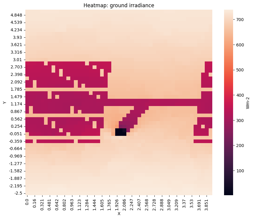
# Create a pivot table to reshape data into a grid
heatmap_data = resultsDF.pivot_table(index='y', columns='x', values='Wm2Front', aggfunc='mean')
plt.figure(figsize=(10, 8))
#plt.imshow(heatmap_data,  aspect='auto', origin='lower')  # imshow doesn't preserve correct x and y coordinates.
#plt.colorbar(label='Wm-2')
ax = sns.heatmap(heatmap_data, cbar_kws={'label': 'Wm-2'})
ax.invert_yaxis()
plt.xlabel('X')
plt.ylabel('Y')
plt.title('Heatmap: ground irradiance')
plt.show()
[ ]:
## Deprecated method, but still works.
sensorsx = 20
startgroundsample=-module.scenex
spacingbetweensamples = module.scenex/(sensorsx-1)

for i in range (0, sensorsx): # Will map 20 points
    frontscan, backscan = analysis.moduleAnalysis(scene, sensorsy=sensorsy)
    groundscan = frontscan
    groundscan['zstart'] = 0.05  # setting it 5 cm from the ground.
    groundscan['zinc'] = 0   # no tilt necessary.
    groundscan['yinc'] = pitch/(sensorsy-1)   # increasing spacing so it covers all distance between rows
    groundscan['xstart'] = startgroundsample + i*spacingbetweensamples   # increasing spacing so it covers all distance between rows
    analysis.analysis(octfile, simulationname+"_groundscan_"+str(i), groundscan, backscan)  # compare the back vs front irradiance
[ ]:
filestarter = "irr_tutorial_11_groundscan_"

filelist = sorted(os.listdir(os.path.join(testfolder, 'results')))
prefixed = [filename for filename in filelist if filename.startswith(filestarter)]
arrayWm2Front = []
arrayMatFront = []
filenamed = []
faillist = []

print('{} files in the directory'.format(filelist.__len__()))
print('{} groundscan files in the directory'.format(prefixed.__len__()))
i = 0  # counter to track # files loaded.

for i in range (0, len(prefixed)):
    ind = prefixed[i].split('_')

    try:
        resultsDF = br.load.read1Result(os.path.join(testfolder, 'results', prefixed[i]))
        arrayWm2Front.append(list(resultsDF['Wm2Front']))
        arrayMatFront.append(list(resultsDF['mattype']))
        filenamed.append(prefixed[i])
    except:
        print(" FAILED ", i, prefixed[i])
        faillist.append(prefixed[i])

resultsdf = pd.DataFrame(list(zip(arrayWm2Front,
                                  arrayMatFront)),
                         columns = ['br_Wm2Front',
                                    'br_MatFront'])
resultsdf['filename'] = filenamed
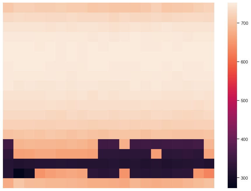
Creating a new dataframe where each element in the front irradiance list is a column. Also transpose and reverse so it looks like a top-down view of the ground.
[ ]:
df3 = pd.DataFrame(resultsdf['br_Wm2Front'].to_list())
reversed_df = df3.T.iloc[::-1]
sns.set(rc={'figure.figsize':(11.7,8.27)})
[68]:
# Plot
print(reversed_df)
ax = sns.heatmap(reversed_df[-20:-1])
ax.set_yticks([])
ax.set_xticks([])
ax.set_ylabel('')
ax.set_xlabel('')
print('')
         0        1        2        3        4        5        6        7   \
19  707.406  717.969  716.894  714.724  714.243  716.414  712.684  712.545
18  729.280  732.414  729.824  730.705  729.512  728.390  732.200  729.413
17  742.290  741.332  741.132  742.073  740.483  742.423  740.617  742.121
16  748.540  749.139  750.334  747.030  746.692  748.511  748.210  747.987
15  751.114  750.602  750.646  748.215  751.154  750.184  750.756  748.963
14  750.900  751.425  750.603  751.448  750.752  749.719  750.619  749.944
13  749.895  750.598  750.358  750.608  749.556  748.857  749.798  748.299
12  749.067  747.934  746.706  748.213  748.873  747.933  745.351  747.451
11  747.113  743.653  745.578  743.618  744.040  745.298  742.976  745.138
10  740.553  740.609  740.436  740.262  741.033  741.978  740.426  741.833
9   737.209  736.845  736.907  736.815  737.291  736.247  734.540  736.351
8   729.293  729.673  727.995  728.887  726.439  725.763  728.758  727.641
7   719.901  718.717  720.173  718.191  716.884  718.772  719.067  718.369
6   700.821  702.329  705.662  701.864  707.937  704.963  700.293  704.312
5   354.341  683.318  687.082  686.330  686.340  684.015  687.402  684.329
4   334.167  662.397  664.277  668.186  670.255  664.270  664.053  663.075
3   320.988  314.571  319.350  321.853  321.258  321.913  320.597  319.688
2   320.926  273.219  294.420  647.285  657.277  664.323  668.472  664.876
1   673.899  704.114  693.208  692.315  687.508  688.551  685.345  681.715
0   707.498  716.469  715.741  713.949  716.359  714.613  711.151  711.483

         8        9        10       11       12       13       14       15  \
19  705.832  708.720  703.669  704.252  702.321  708.024  718.406  706.891
18  728.908  729.055  725.850  730.129  726.288  727.500  728.547  727.856
17  741.224  739.863  738.964  740.845  741.500  740.430  742.609  745.785
16  745.745  749.318  745.715  748.944  750.367  749.119  747.044  747.491
15  751.969  750.249  750.950  751.556  751.332  749.325  750.176  751.702
14  751.767  751.910  751.030  751.151  750.852  751.570  751.093  751.438
13  751.435  751.356  749.836  749.849  749.996  750.831  750.609  749.603
12  748.000  748.337  748.766  749.181  748.254  747.095  749.462  748.451
11  746.259  744.259  743.422  744.654  746.670  745.473  746.861  745.804
10  738.829  742.371  740.733  741.055  742.475  742.264  742.060  740.075
9   736.462  736.461  735.780  736.916  736.081  738.540  737.089  737.146
8   729.293  728.309  727.202  729.124  728.198  727.733  730.143  729.315
7   716.004  717.708  716.707  719.645  717.529  718.759  718.789  716.356
6   700.026  698.568  701.876  701.915  703.323  697.521  703.071  702.413
5   675.622  352.690  353.954  680.402  350.238  352.881  350.218  352.422
4   659.245  329.629  330.931  328.748  328.929  327.717  656.867  326.471
3   319.938  319.540  320.286  316.757  318.837  315.101  319.000  312.704
2   329.639  324.359  326.718  646.582  322.878  321.502  322.878  320.654
1   676.957  676.866  674.528  670.076  685.064  677.959  674.577  678.735
0   705.578  705.871  701.008  706.876  706.066  704.624  707.191  707.824

         16       17       18       19
19  708.602  709.554  715.373  721.070
18  729.540  730.513  730.164  729.620
17  742.639  742.209  742.780  741.877
16  749.018  746.404  747.755  746.784
15  749.695  751.076  750.510  751.580
14  752.223  750.664  750.881  751.237
13  751.574  749.701  750.096  750.593
12  746.353  750.063  749.250  748.708
11  745.252  744.550  745.143  746.247
10  740.399  740.694  742.419  740.563
9   736.811  735.837  735.107  737.445
8   727.679  725.720  726.642  728.830
7   718.192  717.113  720.348  718.582
6   701.093  699.885  701.115  703.428
5   354.495  352.973  358.208  686.067
4   330.890  334.090  328.851  664.724
3   317.191  319.022  320.305  314.738
2   327.450  328.641  648.727  629.784
1   680.499  686.356  691.963  699.706
0   710.695  708.237  712.785  715.473
4. Adding different Albedo Sections#
Add a surface (just like we added the pillars) with a specific reflectivity to represent different albedo sections. In the image, we can see that the albedo between the crops is different than the crop albedo. Let’s assume that the abledo between the crops is higher than the crop’s albedo which wa previuosly set a 0.2.
[ ]:
name='Center_Grass'
carpositionx=-2
carpositiony=-1
text='! genbox white_EPDM CenterPatch 28 12 0.1 | xform -t -14 2 0'.format(carpositionx, carpositiony)
customObject = demo.makeCustomObject(name,text)
scene.appendtoScene(customObject)

octfile = demo.makeOct(demo.getfilelist())
Viewing with rvu: