1 - Introductory Example: Fixed-Tilt simple setup#
This jupyter journal will walk us through the creation of the most basic fixed-tilt simulation possible with bifacial_radiance. We will simulate a 1-up landscape system over a white rooftop.
Steps include:
Create a folder for your simulation, and Load bifacial_radiance
Create a Radiance Object
Set the Albedo
Download Weather Files
Generate the Sky
Define a Module type
Create the scene
Combine Ground, Sky and Scene Objects
Analyze and get results
Visualize scene options
1. Create a folder for your simulation, and load bifacial_radiance#
[1]:
import os
testfolder = os.path.abspath(r'..\..\bifacial_radiance\TEMP\Demo1')

print ("Your simulation will be stored in %s" % testfolder)
Your simulation will be stored in C:\Users\sayala\Documents\GitHub\bifacial_radiance\bifacial_radiance\TEMP\Demo1
Load bifacial_radiance
[2]:
from bifacial_radiance import *

import numpy as np
2. Create a Radiance Object#
[3]:
demo = RadianceObj('bifacial_example',testfolder)
path = C:\Users\sayala\Documents\GitHub\bifacial_radiance\bifacial_radiance\TEMP\Demo1
Making path: images
Making path: objects
Making path: results
Making path: skies
Making path: EPWs
Making path: materials
This will create all the folder structure of the bifacial_radiance Scene in the designated testfolder in your computer, and it should look like this:

3. Set the Albedo#
If a number between 0 and 1 is passed, it assumes it’s an albedo value. For this example, we want a high-reflectivity rooftop albedo surface, so we will set the albedo to 0.62
[4]:
albedo = 0.62
demo.setGround(albedo)
To see more options of ground materials available (located on ground.rad), run this function without any input.
4. Download and Load Weather Files#
There are various options provided in bifacial_radiance to load weatherfiles. getEPW is useful because you just set the latitude and longitude of the location and it donwloads the meteorologicla data for any location.
[5]:
epwfile = demo.getEPW(lat = 37.5, lon = -77.6)
Getting weather file: USA_VA_Richmond.Intl.AP.724010_TMY.epw
 ... OK!
The downloaded EPW will be in the EPWs folder.
To load the data, use readWeatherFile. This reads EPWs, TMY meterological data, or even your own data as long as it follows TMY data format (With any time resoultion).
[6]:
# Read in the weather data pulled in above.
metdata = demo.readWeatherFile(epwfile)
Saving file EPWs\epw_temp.csv, # points: 8760
5. Generate the Sky.#
Sky definitions can either be for a single time point with gendaylit function, or using gencumulativesky to generate a cumulativesky for the entire year.
[7]:
fullYear = True
if fullYear:
    demo.genCumSky(demo.epwfile) # entire year.
else:
    demo.gendaylit(metdata,4020)  # Noon, June 17th (timepoint # 4020)
message: There were 4255 sun up hours in this climate file
Total Ibh/Lbh: 0.000000
The method gencumSky calculates the hourly radiance of the sky hemisphere by dividing it into 145 patches. Then it adds those hourly values to generate one single cumulative sky. Here is a visualization of this patched hemisphere for Richmond, VA, US. Can you deduce from the radiance values of each patch which way is North?
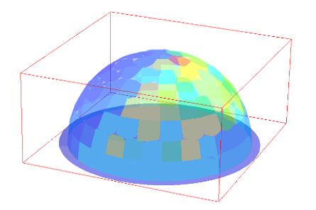
Answer: Since Richmond is in the Northern Hemisphere, the modules face the south, which is where most of the radiation from the sun is coming. The north in this picture is the darker blue areas.
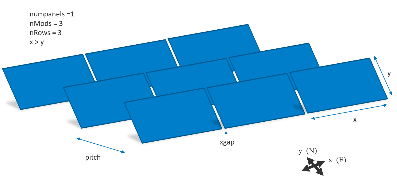
6. DEFINE a Module type#
You can create a custom PV module type. In this case we are defining a module named “Prism Solar Bi60”, in landscape. The x value defines the size of the module along the row, so for landscape modules x > y. This module measures y = 0.984 x = 1.695.
You can specify a lot more variables in makeModule like cell-level modules, multiple modules along the Collector Width (CW), torque tubes, spacing between modules, etc.
Reffer to the Module Documentation and read the following jupyter journals to explore all your options.
[8]:
module_type = 'Prism Solar Bi60 landscape'
demo.makeModule(name=module_type,x=1.695, y=0.984)
Module Name: Prism_Solar_Bi60_landscape
Module file did not exist before, creating new module file
Module Prism Solar Bi60 landscape successfully created
[8]:
{'x': 1.695,
 'y': 0.984,
 'scenex': 1.705,
 'sceney': 0.984,
 'scenez': 0.15,
 'numpanels': 1,
 'bifi': 1,
 'text': '! genbox black Prism_Solar_Bi60_landscape 1.695 0.984 0.02 | xform -t -0.8475 -0.492 0 -a 1 -t 0 0.984 0',
 'modulefile': 'objects\\Prism_Solar_Bi60_landscape.rad',
 'offsetfromaxis': 0,
 'xgap': 0.01,
 'ygap': 0.0,
 'zgap': 0.1,
 'cellModule': None,
 'torquetube': {'bool': False,
  'diameter': 0.1,
  'tubetype': 'Round',
  'material': 'Metal_Grey'}}
In case you want to use a pre-defined module or a module you’ve created previously, they are stored in a JSON format in data/module.json, and the options available can be called with printModules:
[9]:
availableModules = demo.printModules()
Available module names: ['Prism Solar Bi60', '2upTracker', 'test', 'Prism Solar Bi60 landscape', 'cellModule', 'Custom Tracker Module', 'SilvanaModule']
7. Make the Scene#
The sceneDicitonary specifies the information of the scene, such as number of rows, number of modules per row, azimuth, tilt, clearance_height (distance between the ground and lowest point of the module), pitch or gcr, and any other parameter.
Reminder: Azimuth gets measured from N = 0, so for South facing modules azimuth should equal 180 degrees
[10]:
sceneDict = {'tilt':10,'pitch':3,'clearance_height':0.2,'azimuth':180, 'nMods': 3, 'nRows': 3}
To make the scene we have to create a Scene Object through the method makeScene. This method will create a .rad file in the objects folder, with the parameters specified in sceneDict and the module created above.
[11]:
scene = demo.makeScene(module_type,sceneDict)
8. COMBINE the Ground, Sky, and the Scene Objects#
Radiance requires an “Oct” file that combines the ground, sky and the scene object into it. The method makeOct does this for us.
[12]:
octfile = demo.makeOct(demo.getfilelist())
Created bifacial_example.oct
[13]:
demo.getfilelist()
[13]:
['materials\\ground.rad',
 'skies\\cumulative.rad',
 'objects\\Prism_Solar_Bi60_landscape_0.2_3_10_3x3_origin0,0.rad']
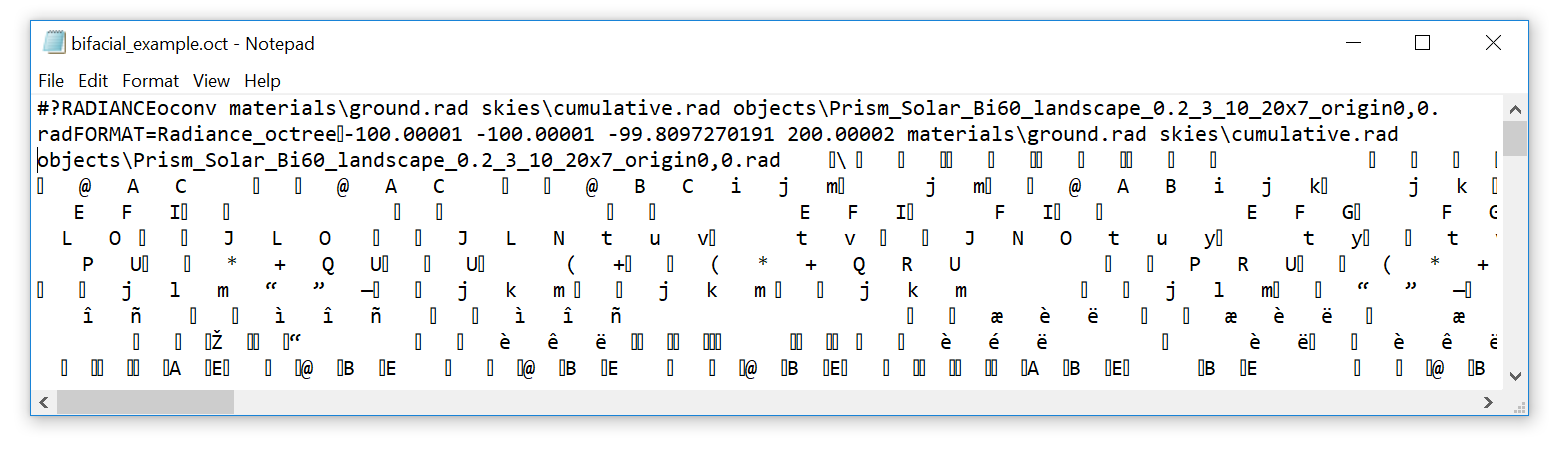
This is how the octfile looks like (** broke the first line so it would fit in the view, it’s usually super long)
9. ANALYZE and get Results#
Once the octfile tying the scene, ground and sky has been created, we create an Analysis Object. We first have to create an Analysis object, and then we have to specify where the sensors will be located with moduleAnalysis.
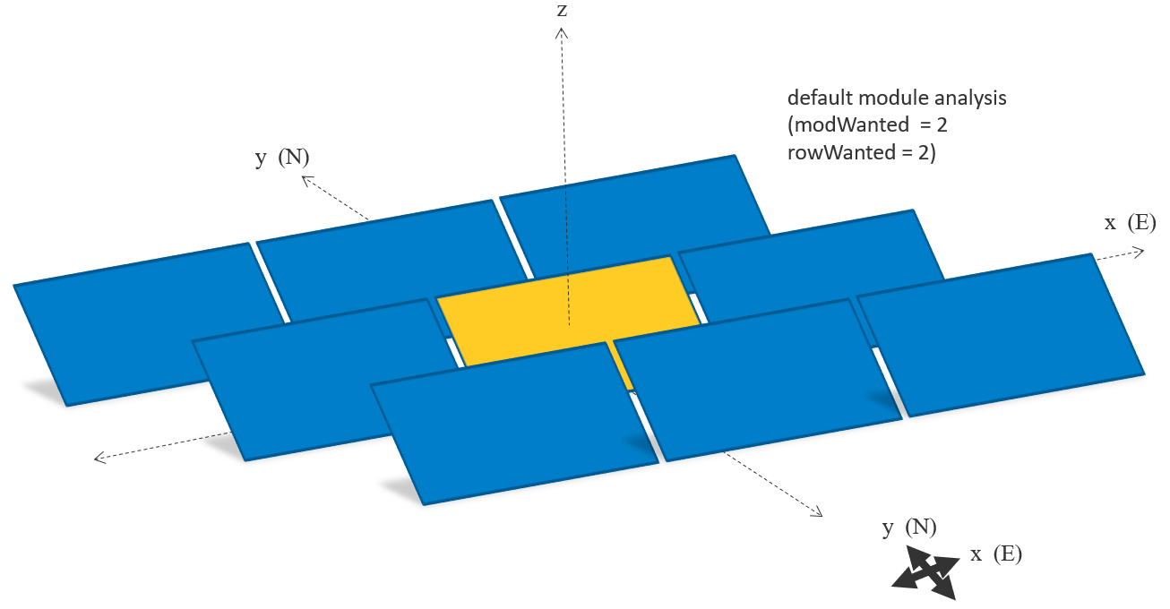
Let’s query the cente rmodule (default)
First let’s create the Analysis Object
[14]:
analysis = AnalysisObj(octfile, demo.basename)
Then let’s specify the sensor location. If no parameters are passed to moduleAnalysis, it will scan the center module of the center row:
[15]:
frontscan, backscan = analysis.moduleAnalysis(scene)
The frontscan and backscan include a linescan along a chord of the module, both on the front and back.
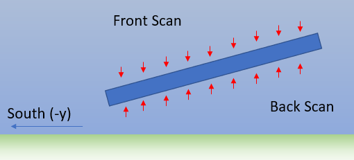 Analysis saves the measured irradiances in the front and in the back on the results folder.
[16]:
results = analysis.analysis(octfile, demo.basename, frontscan, backscan)
Linescan in process: bifacial_example_Front
Linescan in process: bifacial_example_Back
Saved: results\irr_bifacial_example.csv
The results are also automatically saved in the results folder. Some of our input/output functions can be used to read the results and work with them, for example:
[17]:
load.read1Result('results\irr_bifacial_example.csv')
[17]:
| x | y | z | rearZ | mattype | rearMat | Wm2Front | Wm2Back | Back/FrontRatio | |
|---|---|---|---|---|---|---|---|---|---|
| 0 | 4.746980e-17 | -3.876203e-01 | 0.277087 | 0.187087 | a1.1.a0.Prism_Solar_Bi60_landscape.6457 | a1.1.a0.Prism_Solar_Bi60_landscape.2310 | 1534932.0 | 375901.6 | 0.244898 |
| 1 | 3.560235e-17 | -2.907152e-01 | 0.294174 | 0.204174 | a1.1.a0.Prism_Solar_Bi60_landscape.6457 | a1.1.a0.Prism_Solar_Bi60_landscape.2310 | 1535284.0 | 315923.7 | 0.205775 |
| 2 | 2.373490e-17 | -1.938102e-01 | 0.311261 | 0.221261 | a1.1.a0.Prism_Solar_Bi60_landscape.6457 | a1.1.a0.Prism_Solar_Bi60_landscape.2310 | 1535616.0 | 247375.7 | 0.161092 |
| 3 | 1.186745e-17 | -9.690508e-02 | 0.328348 | 0.238348 | a1.1.a0.Prism_Solar_Bi60_landscape.6457 | a1.1.a0.Prism_Solar_Bi60_landscape.2310 | 1535949.0 | 204295.9 | 0.133010 |
| 4 | -1.232595e-32 | 5.551115e-17 | 0.345435 | 0.255435 | a1.1.a0.Prism_Solar_Bi60_landscape.6457 | a1.1.a0.Prism_Solar_Bi60_landscape.2310 | 1536281.0 | 192051.9 | 0.125011 |
| 5 | -1.186745e-17 | 9.690508e-02 | 0.362522 | 0.272522 | a1.1.a0.Prism_Solar_Bi60_landscape.6457 | a1.1.a0.Prism_Solar_Bi60_landscape.2310 | 1536613.0 | 198235.5 | 0.129008 |
| 6 | -2.373490e-17 | 1.938102e-01 | 0.379609 | 0.289609 | a1.1.a0.Prism_Solar_Bi60_landscape.6457 | a1.1.a0.Prism_Solar_Bi60_landscape.2310 | 1536945.0 | 225062.7 | 0.146435 |
| 7 | -3.560235e-17 | 2.907152e-01 | 0.396696 | 0.306696 | a1.1.a0.Prism_Solar_Bi60_landscape.6457 | a1.1.a0.Prism_Solar_Bi60_landscape.2310 | 1523884.0 | 264595.0 | 0.173632 |
| 8 | -4.746980e-17 | 3.876203e-01 | 0.413783 | 0.323783 | a1.1.a0.Prism_Solar_Bi60_landscape.6457 | a1.1.a0.Prism_Solar_Bi60_landscape.2310 | 1523930.0 | 316402.1 | 0.207622 |
As can be seen in the results for the Wm2Front and WM2Back, the irradiance values are quite high. This is because a cumulative sky simulation was performed on step 5 , so this is the total irradiance over all the hours of the year that the module at each sampling point will receive. Dividing the back irradiance average by the front irradiance average will give us the bifacial gain for the year:

Assuming that our module from Prism Solar has a bifaciality factor (rear to front performance) of 90%, our bifacial gain is of:
[18]:
bifacialityfactor = 0.9
print('Annual bifacial ratio: %0.2f ' %( np.mean(analysis.Wm2Back) * bifacialityfactor / np.mean(analysis.Wm2Front)) )
Annual bifacial ratio: 0.15
ANALYZE and get Results for another module#
You can select what module you want to sample.
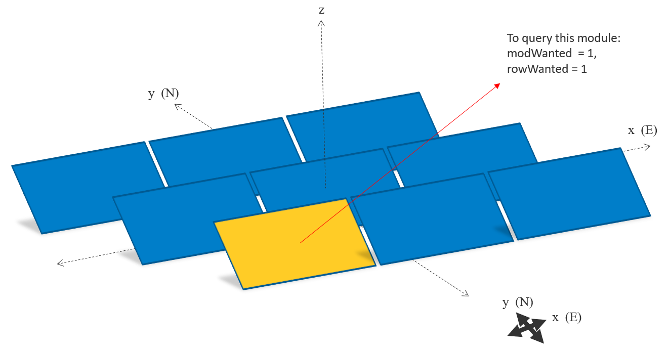
[19]:
modWanted=1
rowWanted=1
sensorsy=4
resultsfilename = demo.basename+"_Mod1Row1"

frontscan, backscan = analysis.moduleAnalysis(scene, modWanted = modWanted, rowWanted=rowWanted, sensorsy=sensorsy)
results = analysis.analysis(octfile, resultsfilename, frontscan, backscan)
Linescan in process: bifacial_example_Mod1Row1_Front
Linescan in process: bifacial_example_Mod1Row1_Back
Saved: results\irr_bifacial_example_Mod1Row1.csv
[20]:
load.read1Result('results\irr_bifacial_example_Mod1Row1.csv')
[20]:
| x | y | z | rearZ | mattype | rearMat | Wm2Front | Wm2Back | Back/FrontRatio | |
|---|---|---|---|---|---|---|---|---|---|
| 0 | -1.705 | -3.290715 | 0.294174 | 0.204174 | a0.0.a0.Prism_Solar_Bi60_landscape.6457 | a0.0.a0.Prism_Solar_Bi60_landscape.2310 | 1534030.0 | 307095.8 | 0.200189 |
| 1 | -1.705 | -3.096905 | 0.328348 | 0.238348 | a0.0.a0.Prism_Solar_Bi60_landscape.6457 | a0.0.a0.Prism_Solar_Bi60_landscape.2310 | 1533973.0 | 282989.9 | 0.184482 |
| 2 | -1.705 | -2.903095 | 0.362522 | 0.272522 | a0.0.a0.Prism_Solar_Bi60_landscape.6457 | a0.0.a0.Prism_Solar_Bi60_landscape.2310 | 1533897.0 | 339068.1 | 0.221050 |
| 3 | -1.705 | -2.709285 | 0.396696 | 0.306696 | a0.0.a0.Prism_Solar_Bi60_landscape.6457 | a0.0.a0.Prism_Solar_Bi60_landscape.2310 | 1533821.0 | 392297.6 | 0.255765 |
10. View / Render the Scene#
If you used gencumsky or gendaylit, you can view the Scene by navigating on a command line to the folder and typing:
***objview materials:nbsphinx-math:ground.rad objects:nbsphinx-math:Prism_Solar_Bi60_landscape_0.2_3_10_20x7_origin0,0.rad***
This objview has 3 different light sources of its own, so the shading is not representative.
ONLY If you used gendaylit , you can view the scene correctly illuminated with the sky you generated after generating the oct file, with
rvu -vf views:nbsphinx-math:`front`.vp -e .01 bifacial_example.oct
The rvu manual can be found here: manual page here: http://radsite.lbl.gov/radiance/rvu.1.html
Or you can also use the code below from bifacial_radiance to generate an .HDR rendered image of the scene. You can choose from front view or side view in the views folder:
[21]:
# Make a color render and falsecolor image of the scene.
analysis.makeImage('side.vp')
analysis.makeFalseColor('side.vp')
Generating visible render of scene
Generating scene in WM-2. This may take some time.
Saving scene in false color
This is how the False Color image stored in images folder should look like:

Files are saved as .hdr (high definition render) files. Try LuminanceHDR viewer (free) to view them, or https://viewer.openhdr.org/